
|
Main themes |
Sub themes |
Description / Contents |
| 1.1 Introduction to field course | Introduction to the nature and purpose of undertaken research. | |
| 1.2 Introduction to Plymouth | Location and background to coastal waters around Plymouth. | |
| 2. Geological/geophysical | The geological analysis aimed to link the marine research with large scale tectonic properties; and how this has shaped the current sea bed and surrounding geography. | |
| 2.1 Geophysical analysis | Side scan sonar and boomer transects. Geological field data. | |
| 2.2 Geological analysis | Analysis of surrounding on shore geology to help understand the marine geology. | |
| 3. Estuarine analysis | To develop an understanding as to how the Tamar estuary acts as a transition zone between the fresh water input at the head of the estuary to to coastal sea. | |
| 3.1 Physical analysis | CTD, tranmissometer and fluorometer profiles. TS (Temperature Salinity) profiles. Secchi disk depths. | |
| 3.2 Chemical analysis |
Main nutrient (silica, phosphorous and nitrate) concentrations. Chlorophyll concentrations. Oxygen saturation. |
|
| 3.3 Biological analysis | Zooplankton net data and phytoplankton data. | |
| 4. Offshore research |
The offshore research aimed to explore the effect of Hand Deeps rock on mixing processes and the effect the mixing process had on both the biological and chemical properties. |
|
| 5. References | Reference list. | |
Abstract
|
The Tamar estuary and the associated offshore waters were surveyed extensively between 29th June 2005 and 13th July using a range of survey vessels. This survey was carried out to determine how the physical and chemical properties interacted to influence the distribution of biology in the estuary. The offshore survey was carried out to determine the influence of Hand Deeps rocks on the mixing of the water columns and tidal currents. An investigation into the geology of the estuarine bed and outcrops of the surrounding area was carried out over several days. This was to determine whether the geology of the region effects the physical and chemical properties of the estuary, and therefore indirectly effecting the biological communities. The data recorded suggested that the stratification of the Tamar estuary is dominated by the discharge of freshwater from the Tamar estuary. There was also a suggestion that extensive mixing took place at the Narrows due to the bottleneck properties of these locations. This extensive mixing was shown by both the ADCP data and the homogenous nature of the water column at this point. The data suggested that the distribution of phytoplankton in the estuary is controlled by the extent of the stratification of the water column and is not nutrient limited. This is shown by the fact that the euphotic depth is deeper than the pycnocline throughout the estuary. The offshore survey showed that the presence of Hand Deeps rocks did influence the mixing and hence the chemical and biological abundances of the surrounding water body. This influence was shown by satellite images to be highly changeable in its extents depending on the weather conditions. |
1.1 Introduction to field course
As guests of Plymouth University we spent 2 weeks from 30th June to 13th July, investigating the physical, chemical and biological properties of Plymouth Sound. Group 7 spent 4 days on the water taking samples and collecting data which was later analysed in the labs. The results of the data, combined with data from 11 other groups from Southampton University, are displayed on this web site.
The site has been divided into sections to convey the information logically: Geological properties of the sea bed and surrounding area; physical, chemical and biological properties of the estuary; and lastly an investigation into how the presence of underwater rock outcrops influence the structure and properties of the water column in offshore surrounding waters.
Plymouth harbour lies at the boundary between Devon and Cornwall, South-west England. The harbour is situated at the end of three rivers the Tamar, Lynher and the Tavy. Together these rivers drain much of Devon and Cornwall and form the largest estuarine system in south west England. The area contains 3 harbour authorities, five international marinas as well as 26 boat yards, 4 local authorities and 2 county councils.
One of the largest and most obvious anthropogenic affects on Plymouth has been a result of the use of the area by the Royal Navy. The Royal Navy has been connected to the area since the Spanish Armada in 1588. The Naval base construction commenced in 1689 and now HMNB Devonport stretches over 650 acres, 4 miles of waterfront and is the largest naval base in Western Europe. There are over 5000 annual ship movements within the harbor due to Devonport’s existence.
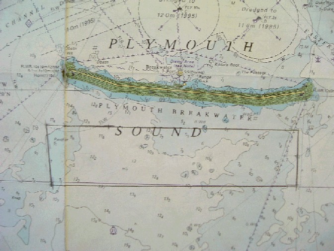
This study aims to provide an independent study into the coastal waters in and around Plymouth harbour including the riverine inputs to the estuary and the offshore sinks. The location of the area of study can be seen in figure 1.2.1
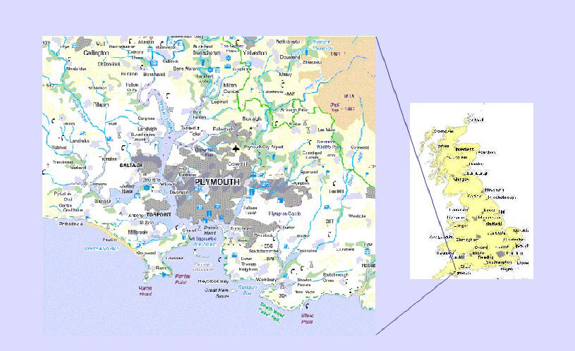
Figure 1.2.1 The location of the study.
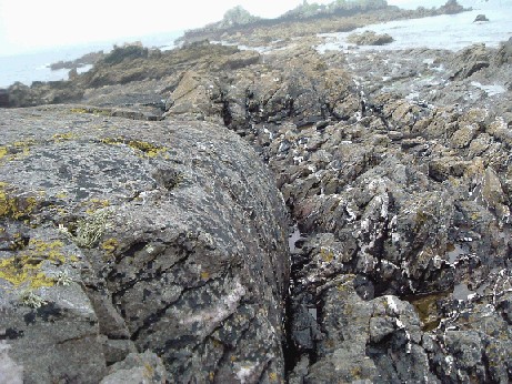
The geological analysis is divided into two sections, geophysical and geological. Group 7's geological field trip took place on Saturday 2 July 2005 at Heybrook Bay, Plymouth. Here we studied the geological structure of Renney Point and the surrounding area of Heybrook Bay to give us a geological overview of the area and an understanding of the influence of the bedforms on the estuary. The following day (Sunday 3 July 2005), Group 7 investigated the estuarine bed using side scan sonar aboard The Nat West II surveying vessel, the results of which are detailed below.
The geology of a region influences the chemical and physical properties directly, and therefore the biology indirectly. The sediment type (section 2.2) influences the influx of minerals to the estuary and therefore has a huge impact on the nutrient levels. The bedforms found in the estuarine bed can effect the mixing due to the different sediment types effecting the depth and flow of the river (section 2.1). For example, a body of water over fine sediment will travel faster than a body of water over bedforms. The paleoecology of the estuarine floor will also affect the present day geological structure, i.e. past fluvial channels.
|
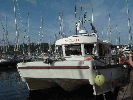
The geophysical survey took place on 3 July 2005, aboard the survey vessel, Nat West II. Unfortunately, the planned survey of the shipwrecks in Whitesands Bay was not possible due to divers on the wreck. Four good side scan sonar tracks were completed in an designated area outside of the breakwater. |
|
|
Figure 2.1.1 The survey vessel Nat West II |
|
|
|
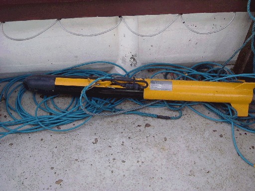
The fish was towed at an approximate depth of 1.5m, 3m from the stern of the ship, at an average speed of 4 knots. The exact chart co-ordinates of the survey lines are recorded in the log book and the side scan sonar analysis. |
| Figure 2.1.2 The fish containing the side scan sonar. | |
|
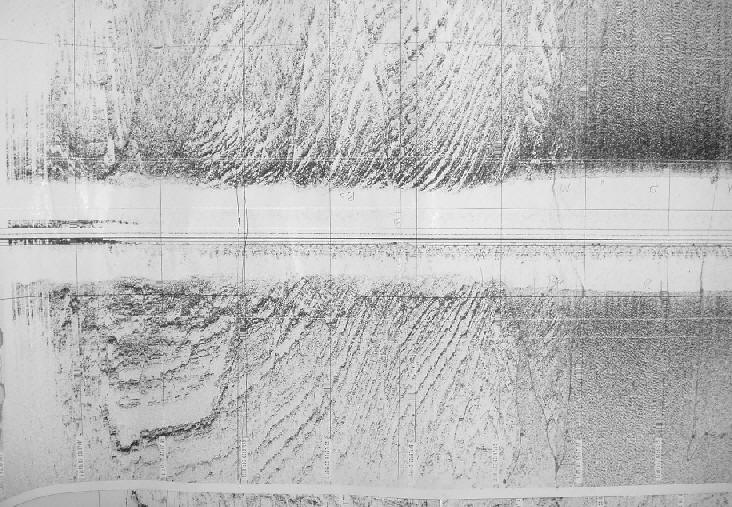
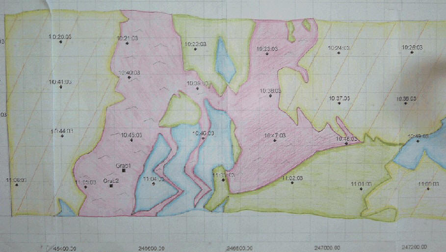
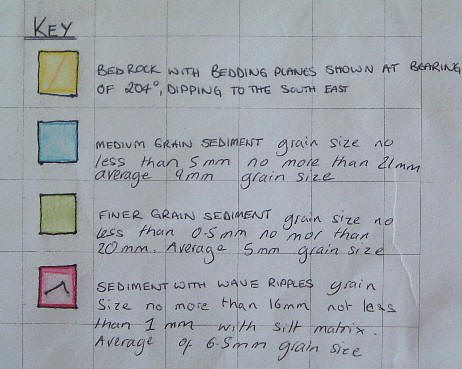
Analysis of the raw data identified four different sediment types including a large area of bedrock (Figure 2.1.3). The bedrock is part of the continental plate and forms the majority of the plot. The bedding planes found in the bedrock identify the rock as sedimentary bed with a bearing of 204o and dipping to the south east. This also relates to the geological analysis of the section 2.2 where the outcrops observed were sedimentary sand and silt stone. So therefore a hypothesis that the bedrock found in the estuary was from the same formation can be formed. |
|
|
Figure 2.1.3 A section of the original profile of sea bed as produced by the side scan sonar |
|
|
|
The three sediment types were identified as 1. Fine grained. Mean grain size 0.5mm>GS<20mm, average 5mm. 2. Medium grained. Mean grain size 5mm>GS<21mm, average 9mm. 3. Sediment with wave ripples. Mean grain size 16mm>GS>1mm, with silt matrix, average of 6.5mm grain size. The side scan raw data showed a large shadow following a pronounced ripple, thus indicating that the stoss is longer than the lee, resulting in the ripple being influenced by a unidirectional flow i.e. wave. The ripples were identified as wave induced features rather than current induced features as the waves were asymmetrical. The waves also appeared to be bifurcating rather than parallel, a further identifying feature of wave induced ripples.
|
|
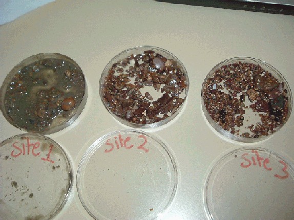
Figure 2.1.4. Sediment collected from sea bed, dried and stored in petri dishes |
|
|
The majority of the sediment was deposited along a tract running perpendicular to our survey lines, from north to south. This area corresponds to a deeper channel area in relation to the sea surface, which may be due to an underlying river valley carved out by a river which once flowed at a time of lower sea level.
The channel was easily identified on the admiralty chart, as it is situated between two large bands of bedrock, indicated on the chart by two areas of shallower sea floor, marked in light blue. Figure 2.1.5 |
|
|
Figure 2.1.5 Side scan sonar interpretation of sediment type with key. |
|
|
|
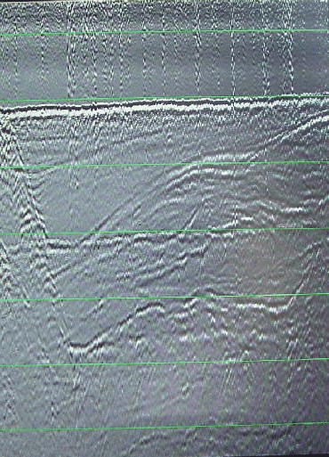
Use of the boomer enabled identification of the river valleys beneath the current sediment layers. This was up to 50m below the present sea floor. Data from the boomer appeared to correlate with the side scan sonar data, as there is an obvious channel between two sections of bedrock. |
|
Figure 2.1.6 . Image of boomer screen illustrating paleo-river channel. |
|
|
|
|
Figure 2.1.7. Location of side scan sonar transect |
From the side scan sonar raw data several sample locations were decided on. The locations were linked with the the three sediment types, not including the bedrock, that where obvious on the side scan. The equipment initially used was the Van Veen grab, but problems were encountered with pre-tripping and the jaws of the grab being jammed open by large rock fragments, therefore the remaining samples were taken using the pipe dredge. Consequently, instead of taking a discrete sample at a specific site, the sediment collected was taken from a larger area and was therefore was less quantitative than was first planned.
| Site 1 (50o 19.700’ N 4o 09.500’W) Figure 2.1.4 |
This Van Veen grab sample consisted of a fine matrix of size <1/16mm and is therefore a silt type sediment. Also there was gravel present, with sizes ranging from 1-16mm. The gravel was well rounded, and therefore had been subject to extensive erosion. A16mm white annelid was collected at this site, also present in the grab were various shell fragments about 2mm in size. This site corresponds to the red section of the side scan sonar processed chart. |
|
Site 2 sample – Start: 50o 19.8’N 4o 08.8’W Stop: 50o 19.7’N 4o 08.0’W |
In this pipe dredge the sediment was of a coarser grain size and contained various rock fragments ranging in size from 2mm-21 mm. Also present in the dredge were shell fragments from gastropods and ammonites. This site corresponds to the blue section of the side scan sonar processed chart.
|
|
Geofield 3rd July 2005 Location: Renney Point at Heybrook Bay, Plymouth Easting: 49250 Northing: 49770 |
Aims: From the outcrops shown in this area, an idea of the sedimentary structure of the estuarine bed can be obtained. Also, the sedimentary supply to the water can be observed by noting the mineral composition of the sedimentary sequence, which gives a palaeoecological overview. |
Structural Overview –
|
|
|
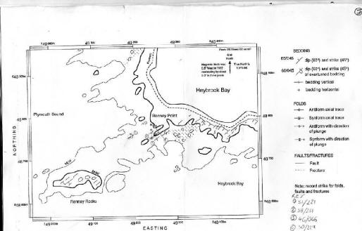
| Figure 2.2.1. A Geological Map of Renney Point at Heybrook Bay, Plymouth showing dips, strikes and bearings of the main geological structures (click graph for larger image) |
|
 |
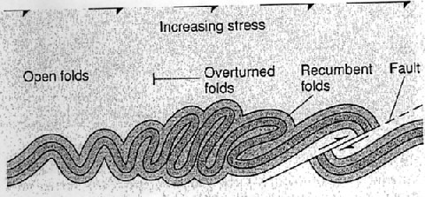 |
| Figure 2.2.3. Diagram of how sedimentary formation occurs under stress | |
| Figure 2.2.2. View of hinge facing south-west, antiform found at Renney Point, Heybrook Bay, Plymouth | |
Figure 2.2.1 shows an outcrop of an antiform fold. The hinge of this fold structure is shown in figure 2.2.2. To the north-west of the hinge line of this antiform, the bedding planes are overturned, which indicates a synform under the surface sediment. Figure 2.2.3 indicates how the formation of this occurred, where the initial fold is the antiform shown in our outcrop. The Figure 2.2.2 shows the top of the top of this fold, the hinge.
Also indicated on the geological map is a major dextral fault with an approximate 5m movement. This fault is also shown through the estuary bed in the side scan raw data sectional area observed by group 5 in the location of 49 000.00N, 24 75 00.00W.
The geology of the estuary can be speculated by observation of the outcrops if the fault and fold structures are also found to be present in the estuarine bed.
Sediment Sequence Overview
|
|
Description < ¼ mm Grain Size :- Medium Sand Matrix Supported Red Matrix with grey breccia and shell clasts
< 1/8 mm Grain Size :- Fine Sand Clast supported, small yellow-grey clasts with same orientation Angular (breccia)
1/16 Grain Size :- Fine grain and Silt matrix Matrix supported with medium clasts Reverse grading Clasts orientated with bed Red Matrix
1/16 mm Grain Size :- coarse silt, red matrix
< 1/16 mm Grain Size :- Silt Few Clasts, smooth red clay composite
<1/16mm Grain Size Large breccia clasts of varying sizes Red Graded bed
|
Analytical View Submarine Little transportation of clasts therefore from local source Marine/ Estuarine Deposit
Terrestrial oxic red soil from erosion following deglaciation Transported by mudflow from meltwaters. Low vegetation Flood Plain deposit
Increased grain size shows sea level rise
River stream deposit. Subaerial Clasts from pre-existing rocks |
Figure 2.2.4 Sedimentary sequence at Renney Point, Heybrook Bay, Plymouth, with analysis.
From the sediment sequence above, a paleoecological hypothesis can be suggested. The bottom bed is the oldest bed, dating back to just after the deglaciation in the Pleociene age. As the sequence decreases in age the increase in grain size also indicates the increase in sea level. The presence of the large flood plain bed, as well as the presence of vast amounts of melt water may have been due to the lack of vegetation causing increased sediment flow. The timing of the Milankovitch cycles tie in with the order of deposition, which suggests that the sequence is post 12,000 year ago.
Estuaries are semi-enclosed bodies of water that tend to have different characteristics than the open sea which they flow into. They are often located in areas of high industry and anthropogenic influence and are used as conduits for wastes and contaminants into the open sea. Alongside this they support a diverse range of flora and fauna that can be largely effected by anthropogenic activities. The aim of this estuarine study was to develop an understanding of how the Tamar estuary acts as a transition zone between the freshwater input at the head of the estuary, to the coastal sea.
Estuarine samples and data were collected by Groups 7 and 8 on 30 June 2005. Group 7 were aboard the Bill Conway and took samples at 6 stations south of the Tamar Bridge. Group 8 were on the RIBs (Ocean Adventure and Coastal Research) and collected data from the head of the estuary to the north of the Tamar Bridge. Table 3.1 gives details of station numbers for both groups and geographical locations.
Group 7 collected data using a CTD, ADCP, Plankton net, secchi disk (see Biology, section 3.3) and a continuous TS probe for surface salinity. Group 8 collected their data on the ribs using a plankton net, a multiprobe and a plastic container for surface samples.
Using this data, along with data collected by other groups, we can build up a profile of chemical, biological and physical properties of the estuary, how these properties change with progression from the head to the mouth and what influences such changes.
Tides on the 30 June 2005 were on neaps, with high water at 1230 GMT and low water at 0630 GMT. Wind speed was 3-5 knots with gusts of up to 10-15 knots, sea state was medium with intermittent rain and 8/8 cloud cover.
|
Table 3.1. A table illustrating the station numbers surveyed with time from RV Bill Conway, Ocean Adventure and Coastal Research (GMT), Latitude and longitude and geographical features. Station Numbers beginning with R were carried out from the Ribs. Stations labelled a-d subsections of the same geographical locations, please refer to figures X and Y. |
|
|
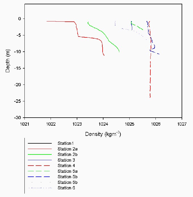
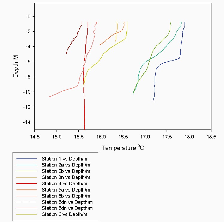
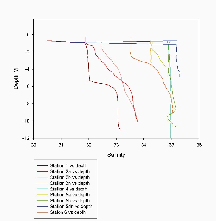
The CTD was used by Group 8 in the Bill Conway only, therefore the following data and interpretation refers only to stations 1 - 6 (see Table 3.1). Samples taken at Stations 1-3 were taken on the flood tide and samples taken at stations 4-6 were taken on the ebb tide. Whilst the changing tide would have had an effect on the water column it is not thought to have encouraged mixing and therefore it is not thought to have had a notable effect on the water samples. Therefore the tide would not have progressed enough to influence the samples as the Tamar has been found to be have a long, slow ebb. (Uncles et al. 1985) As can be seen from figure 3.1.2 and figure 3.1.4 the station sampled farthest towards the head of the estuary showed a strong influence by the river end member, with a strong stratification of the water column. There is a layer of less haline, and therefore less dense layer of water down to a depth of 5-6m. There is also a strong thermal stratification of the water column, with the layer influenced by the river end member being 0.7 oC warmer than the bottom marine-dominated layer (see figure 3.1.3). There is also a significant, freshwater surface layer, due to a high discharge from the river end member, caused by a large amount of rainfall in the days before, and during the periods of sampling. There was a decrease in water column stratification with progression towards the mouth of the estuary, due to increasing dominance of the marine end member and the flood tide. The sharp decrease in surface salinity at station 5 seen in figure 3.1.4 was likely due to heavy rainfall at the time of sampling. |
||||||
|
|
|
|
||||
|
Figure 3.1.2. Density against depth from CTD |
Figure 3.1.3. Temperature against depth from CTD |
Figure 3.1.4. Salinity against depth from CTD |
||||
|
The significant decrease in salinity and density, and the more extensive stratification at station 6 shown on figure 3.1.4 and figure 3.1.2, is due to the input of water from the River Cattewater, where sampling took place at the mouth. Figure 3.1.4 shows that the salinity decrease is most evident at the surface. This decrease in salinity, and hence density, is less than that of the samples taken at the furthest point of the estuary and at the mouth of the Lynher River. This is most likely due to their comparative sizes and the level of discharge. The location of station 4 in the Narrows is virtually homogenous, due to increased mixing caused by shear between the layers of fast flowing water in the channel, (see section on ADCP). By comparing the
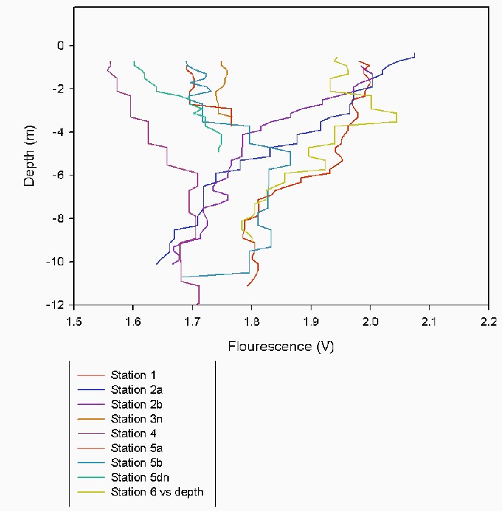
data received from the transmissometer (figure
3.1.5) and the fluorometer (figure 3.1.6), the nature of the
suspended particles could be determined. As can be seen from
Figures 3.1.5 & 3.1.6, most of the suspended
particles in the water column above the pycnocline were recorded by the
fluorometer, and
are therefore perceived to be chlorophyll. This
however is not an indicator of biological activity, as the chlorophyll
molecules may have originated from dead cells. The locations of fluorescence
maxima were at the river water input sites, the Tamar, Lhyner and Cattewater,
which corresponds to the chlorophyll data displayed in section 3.2
chemistry. This was probably due to the input of nutrients at
these points. The fact that there were biological molecules down to the pycnocline is confirmed
by the secchi depth and consequent depth of the euphotic zone (as shown
in figure 3.1.19).
The euphotic zone was always below the pycnocline, with the exception of
Station 1, where the euphotic zone is the same as the depth of the surface
mixed layer. The fast currents at station 4 (the Narrows) caused a
large amount of mixing and the concentration of suspended particle
material was found to be homogenous to the entire water column.
|
||||||
|
|
|
|||||
| Figure 3.1.5 The volume of suspended particulate matter against depth, derived from the tranmissometer on board RV Bill Conway on 30/06/2005. | Figure 3.1.6. Fluorescenceescence against depth, derived from the fluorometer on board RV Bill Conway on 30/06/2005. | |||||
Current Velocity and backscatter
|
Water velocity and backscatter was measured using an Acoustic Doppler Current Profiler (ADCP). This instrument sends out pulses of sound at a frequency of 1200 kHz. The volume of reflected sound or backscatter can help determine the volume of suspended material in the water. The Doppler shift of the sound is then used to determine the speed of the water. The ADCP sends out four acoustic pulses, the speed determined from the return of each of these is then used to calculate the velocity of the water column. This instrument may be used aboard a moving vessel as the velocity is calculated using the sea bed as the stationary reference point.
|
||
|
ADCP transect 1 at station 1a (see Table 3.1, locations of stations), shows the tide coming into the estuary, heading north towards the Tamar Bridge at an average speed of 0.50m/s, which increases with peaks at 0.85m/s as the water reaches the side of the estuary. Transect was started at 08:44 GMT and finished 08:45 GMT, 3 hours and 45 minutes before high water, so the tide was still coming in. The directional velocity ranges from between 45 degrees and 297 degrees, forming a northern heading current. There was some suspended material in the surface picked up by the backscatter, most likely from debris discharged by the ferry. There was also backscatter from the sea floor, where the incoming tide would be disturbing the sediment. The Richardson number for station 1a was 0.31, showing that the water here was stable although only a small perturbation would be required to make it unstable.
|
||
 |
 |
|
|
Figure 3.1.7. An ADCP plot from station 1 to show backscatter. |
Figure 3.1.8. An ADCP plot from station 1 to show velocity magnitude. |
Figure 3.1.9. An ADCP plot from station 1 to show velocity direction. |
|
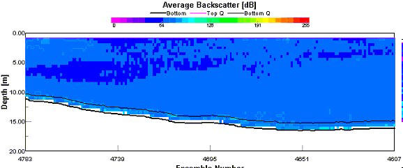
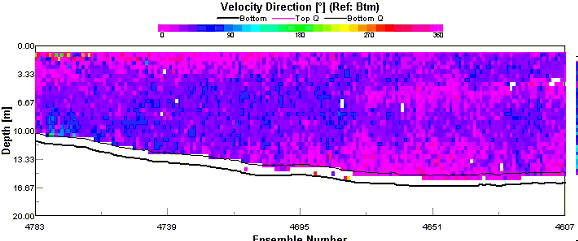
The ADCP transect at station 3, before the narrows showed that the velocity profiles are relatively low, ranging from just above 0.00 to 0.40 m/s in the majority of the channel, with some of the faster flowing water towards the centre (ensemble 231) forming faint vertical columns. The fastest water currents are where the channel gets shallower towards the east side (ensemble 26). Transect was started at 11:07GMT ending at 11:10GMT at the edge of a dock, taken 1 hour and 20 minutes before high water, so the tide was still coming in but at a lower rate. Velocity direction varies greatly between just below 90 degrees and over 300 degrees across the channel, indicating eddies in the water column. Depths below 16 m were not recorded due to the bin size of 0.5m the ADCP uses being too small to reach greater than that depth. The Backscatter shows
layers of different sediment content, higher at the surface and at the
bottom, matching where the velocity direction changes most rapidly.
|
||
 |
 |
 |
|
Figure 3.1.10. An ADCP plot from station 3 to show backscatter. |
Figure 3.1.11. An ADCP plot from station 3 to show velocity magnitude. |
Figure 3.1.12. An ADCP plot from station 3 to show velocity direction. |
|
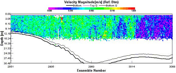
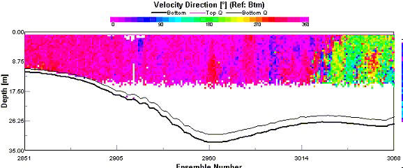
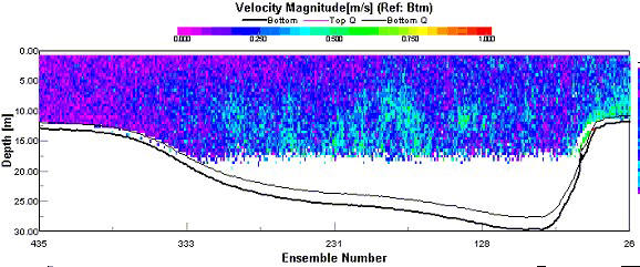
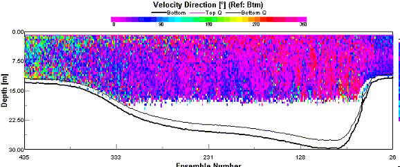
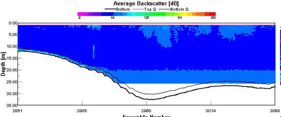
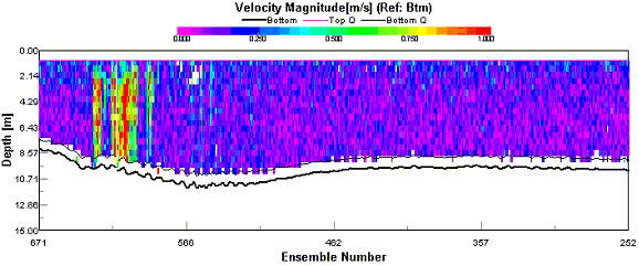
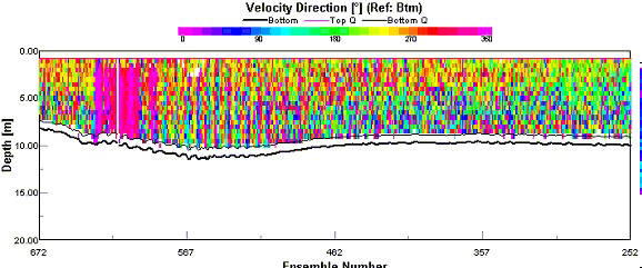
ADCP transect at station 4, the narrows, shows a strong current profile heading north at ~60cm/s throughout the west half of the channel (ensemble 2960 and lower), which changes to a weaker current at ~10cm/s heading south on the eastern side of the channel (ensemble 3030 and higher). This transect was started at 11:28GMT finishing at 11:30 GMT, an hour before high water so the water was approaching slack. The vertical profiles of the water indicate (see ensemble 2960 to 3014) eddying in the narrows, especially where the directional velocity changes from varying around 350-15 degrees to 200-170 degrees. The eddying makes the water much more homogenous which is also shown by how little the salinity and temperature vary with depth (maximum difference of 0.105 ° C and 0.075 salinity) as recorded on the CTD. However, ADCP data from below 16 m was unobtainable due to the depth bin size used being too small (0.5m), leaving a gap where CTD data would be compared. The Richardson number for station 4 was 0.003, showing that the water was unstable to a very high degree.
|
||
 |
|
|
|
Figure 3.1.13. An ADCP plot from station 4 to show backscatter. |
Figure 3.1.14. An ADCP plot from station 4 to show velocity magnitude. |
Figure 3.1.15. An ADCP plot from station 4 to show velocity direction. |
|
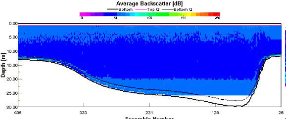
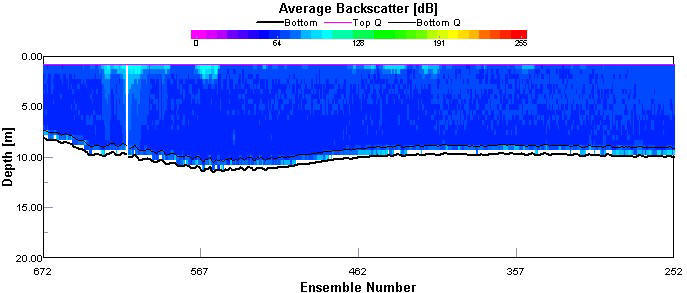
ADCP transect at station 6 shows a slow current speed at an average of 19cm/s until 2 minutes and 27 seconds into the transect (ensemble 618) where the current speed increases to upwards of 80cm/s. This area of high speed current is also high in suspended particulate matter shown on the backscatter, both of which are more than likely due to the River Plym opening into this area called Cattewater. This transect was started at 13:44 GMT and finished at 13:47 GMT, an hour and 15 minutes after the high water so the tide would be going out. CTD data shows a decrease in salinity towards the surface, suggesting the freshwater input was becoming more established. The Richardson number for station 6 was 0.008, showing that the water was unstable to a very high degree.
|
||
 |
 |
 |
|
Figure 3.1.16. An ADCP plot from station 6 to show backscatter. |
Figure 3.1.17. An ADCP plot from station 6 to show velocity magnitude. |
Figure 3.1.18. An ADCP plot from station 6 to show velocity direction. |
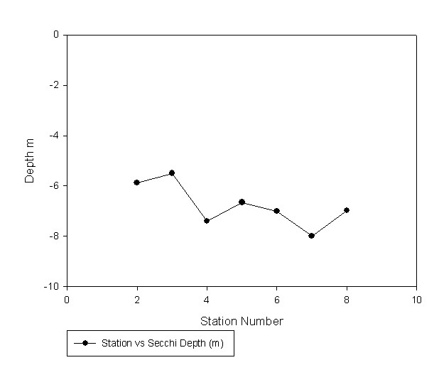
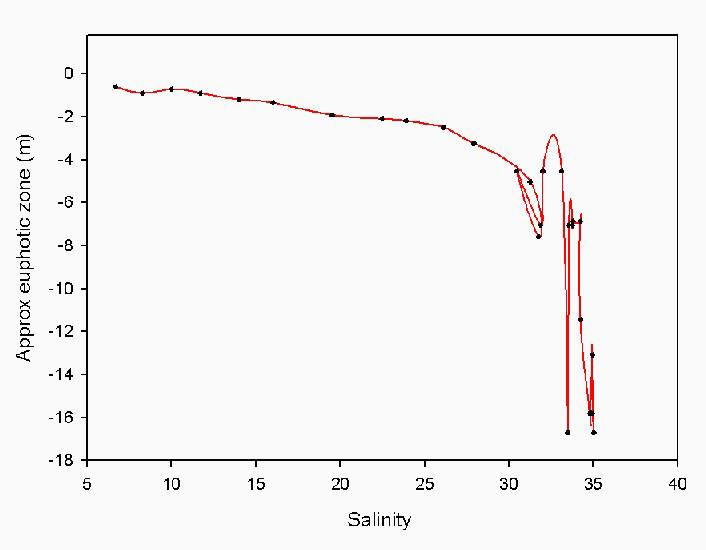
A secchi disk was used to give an indication of depth of the euphotic zone, which is the limit for plant growth in the water column. The disk is lowered into the water until the operator can no longer see a contrast between the black and white segments on the disk surface, this is the secchi depth and this measurement is multiplied by three to give the depth of the euphotic zone.
The secchi disk generally gives quite accurate results, however it’s limitations lie in that it assumes that the properties of the surface water is the same for the whole water column.
From the secchi disk depths the euphotic depth found in the upper estuary between salinities of 6 and 26 was a lot shallower in the water column. This would be the limiting factor for biological activity in the water column, as the water depth when the measurements were recorded in this part of the estuary was 2-4 times the calculated euphotic depth. The shallowness of this euphotic depth was due to the high turbidity of the water column from a high level of river discharge attributed to heavy rainfall in the previous month (3% higher than average using data from the Environment Agency). This high turbidity in the lower estuary has been investigated extensively due to the presence of a turbidity maximum present in summer. This is more evident on spring tides, having a maximum of 2-3kgm-3 of sediment, however on neap tides there is still a turbidity maximum of 0.2kgm-3 (Tattersall et al. 2003). This turbidity maximum was obviously present in the upper estuary due to the very shallow euphotic depth and was a controlling factor on the phytoplankton in the water column at these salinities. The presence of this turbidity maximum could be investigated using a combination of a tranmissometer and a flurometer, however the boats used to access the upper estuary were not equipped with this equipment (see figure 3.1.19)
|
At a salinity of 27, the euphotic zone was deeper than the water depth so the turbidity of the water column would not be a factor in controlling the biology at this point. From a salinity of 27, the euphotic zone was deeper than the pyncoline, explained in full in the section and shown in figure 3.1.2 so it was the euphotic zone, in this part of the estuary, that was the controlling factor of the distribution of the biology in the water column. At a salinity of 33.7 to 34.2, the euphotic depth became a lot shallower. This was due to the location of these salinities (the Narrows), where the water movement was at a maximum (see Current velocity and backscatter). These fast currents have been shown to cause a high level of mixing (see CTD section). These fast currents stirred up a lot of sediment from the estuary bed, which caused the water column to be highly turbid and hence have a shallow euphotic depth, as proved by the data collected in this survey. |
 |
|
Figure 3.1.19 The secchi disk depth throughout the Tamar estuary on 30/06/05 |
Water samples collected on each boat on 30 June 2005 were analysed in the lab the following day to determine the behaviour of nutrients in the estuary. The samples collected were either surface samples from the continuous water sampler (on Bill Conway), or a collection with an open container (on the RIBS). Nitrate, phosphate, silicon, oxygen and chlorophyll were analysed for each water sample using methods detailed in the literature, and estuarine mixing diagrams were constructed for each property. Interpretation of estuarine mixing diagrams gives an indication of whether the nutrients are conservative or non conservative in behaviour, however the limitations in using mixing diagrams includes assumptions that the system is in steady state and can be described by a one dimensional mixing model. It is also assumed that the end member concentrations are constant on a time scale greater than the residence time of the estuary.
|
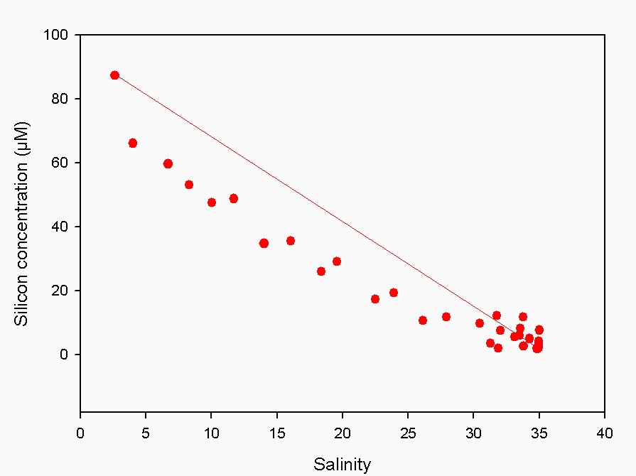
Silicate Silicon displayed non conservative behaviour from the head to the mouth of the estuary, and as the points on the diagram deviate from the Theoretical Dilution Line (TDL) this indicates removal of silicon from the water. The estuarine mixing diagram shows that the points become clustered around the TDL at a salinity of 30 – 35, at the mouth of the estuary below the Tamar bridge. At this point, silicon is no longer being removed or added. The removal of silicon from the waters may be due to both biological and non biological factors. Biological removal of silicon occurs when diatoms utilize silicon for the formation of frustules, therefore the high silicon values and the high chlorophyll values (Figure 3.1.4) found at low salinities at the head of the River Tamar, suggest biological removal. This correlates with the phytoplankton samples taken by group 8 at the head of the river, which shows an abundance of diatoms. Silicon may also be removed chemically by flocculation.
|
|
|
Figure 3.2.1. An estuarine mixing diagram of silicon in the Tamar estuary (click graph for larger image) |
|
|
|
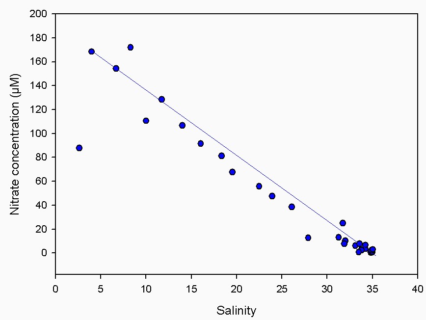
Nitrate Most of the data points on the mixing diagram occurred in a moderately straight line relative to the Theoretical Dilution Line which suggests conservative behaviour. Deviation from the line occurred at low salinity values around 10 – 12, which showed addition and then removal of nitrate. This may be due to the variability in the composition of fresh water entering the estuary, as found in previous studies of the Tamar estuary. Further studies by Morris et al, 1981 found that such fluctuations damped out at higher salinities.
|
|
Figure 3.2.2. An estuarine mixing diagram of nitrate in the Tamar estuary (click graph for larger image) |
|
|
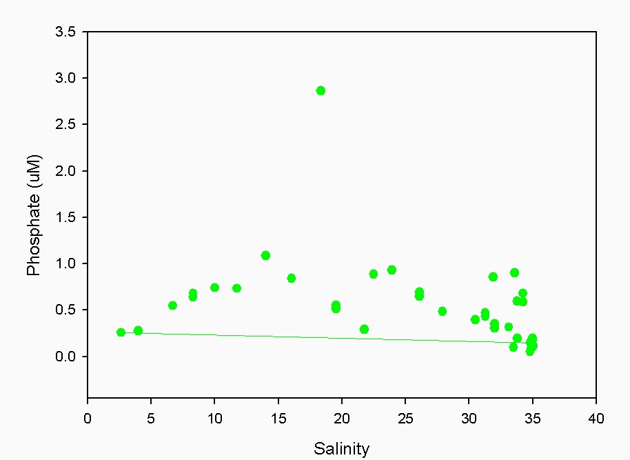
Phosphate. The majority of the points lie above the TDL, which suggests non conservative behaviour (Figure 3.2.3), however it is uncertain as to whether these measurements are accurate. The low phosphate values at the head of the estuary are not consistent with other group's data which indicates that the data may be wrong. Group 11 took phosphate samples at the head of the river the following day and the mixing diagrams showed conservative behaviour. The major points of addition appear to occur at salinities of 14, 24 and 34, which coincide with river inputs and anthropogenic input. Removal of phosphate occurred at the mouth of the estuary (salinity of 35), this may be due to non-biological buffering mechanisms found to be operative within estuarine systems (Morris et al, 1981). One rogue point was recorded at a salinity of 17, showing a value of 2.86 µM, this was most likely due to faulty equipment.
|
|
|
Figure 3.2.3. An estuarine mixing diagram of phosphate in the Tamar estuary (click graph for larger image) |
|
|
|
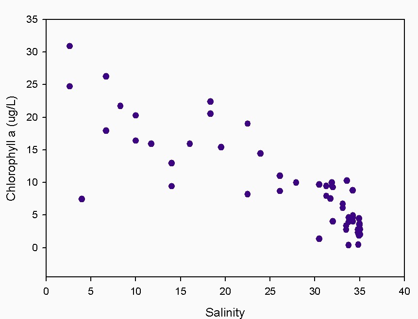
Chlorophyll The high chlorophyll values found at the head of the estuary (Figure 3.2.4) indicate high biomass in that area, with the highest value of chlorophyll (30.9µg/L) found at a salinity of 2.5. Chlorophyll values generally decreased with an increase in salinity from the head to the mouth, this corresponds to the higher values of silicon and nitrate at the head of the estuary. As the phytoplankton utilise the nutrients they are removed from the system and phytoplankton biomass increases. The low chlorophyll values at the mouth of the estuary indicate low phytoplankton biomass which may be due to increased grazing pressure by zooplankton, this was confirmed by the two zooplankton counts carried out at the end members
|
|
Figure 3.2.4 Chlorophyll distribution throughout the Tamar estuary in relation to salinity. |
|
Oxygen The oxygen data collected from the estuarine survey boats was of limited use as a number of errors occurred with sample collection and processing. Firstly, ½ the sample bottles lost their unique numbers, and with the limited facilities available in the field, the unique volume of these bottles could not be determined, rendering them useless. The remaining oxygen samples taken were processed and added to the dissolved oxygen data obtained from the multiprobes on the estuarine RIBs. However the multiprobe data was less accurate due to calibration problems, as atmospheric pressure was influential in the oxygen calculation and another limitation with equipment meant that this could not be measured. Therefore, in order to bring the multiprobe data to a more reasonable level of accuracy, stations with data from both the lab and multiprobe were used to produce a linear scale of the error in the multiprobe readings. This then gave a value of approx. 44 mM which was subtracted from the multiprobe data (blue points on figure 3.2.5) to bring it in line with the lab data (red points on figure 3.2.5). |
|
|
Figure 3.2.5. Oxygen concentrations in the Tamar estuary on 30/06/2005. (Red points are derived from titrations carried out ashore, blue points were in situ measurements from the TS probe).
|
|
|
The calibrated data on figure 3.2.5 does give some insight into the estuary. The results show a high oxygen concentration of around 300 mM at salinity 2, with a sharp decrease in the mid estuary, until a salinity of around 10, where oxygen concentrations increase again. This profile is expected from the spring/summer period due to an oxygen demand exerted in the upper estuary (A.W. Morris et al., 1981). This high demand is partly due to industrial and domestic effluent discharged into the river, as well as phytoplankton, which create the high oxygen concentrations in the estuary mouth, being transported up the estuary and respiring in the more turbid waters (see secchi disk data). There is a decrease in oxygen concentration from salinity values of 23 to 35, as around 23 phytoplankton species are autochthonous and have sufficient nutrients to have a higher growth rate and maximum population compared with the populations in the mouth of the estuary. Oxygen concentrations are also lower in the mouth of the estuary as the phytoplankton are allochthonous and so do not have time to establish a population, instead they are influenced by the tidal currents. The data shows that oxygen is not conservative in the estuary but is rather determined by in situ biological and chemical processes as well as the kinetic limitations of equilibrium in a dynamic system such as the Tamar estuary (A.W. Morris et al., 1981). |
|
|
|
|
||
|
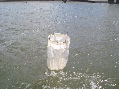
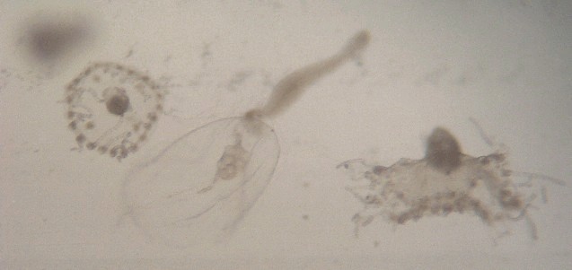
Figure 3.3.1. A photo to illustrate typical plankton samples |
|||
|
|
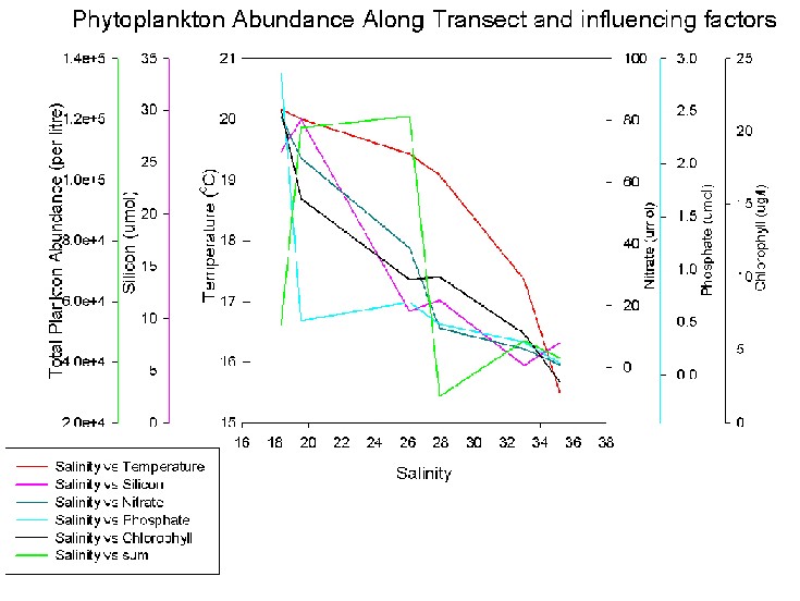
Figure 3.3.2 shows an overall abundance of phytoplankton along the
transect on Phytoplankton is dependent on light,
temperature and nutrients, which decrease from the head to the mouth
of the estuary. The
phytoplankton showed an increase in abundance up to the bridge, where a
decrease occurred. Around
the The chlorophyll data also shown on the graph illustrates that there were more phytoplankton in the water near the head of the estuary. Moving down the estuary nutrients and chlorophyll decrease, this corresponds to the plankton numbers as they utilise the nutrients and hence remove them from the system. This was also indicated by the fluorometer readings shown in section 3.1 (physical properties). |
||
| Figure 3.3.2. A graph showing phytoplankton abundance and influencing factors along transect on 30/06/2005. | |||
| Transmissometer
readings correlated with fluorometer readings indicating chlorophyll,
but not necessarily biological activity. The ADCP can measure current
velocities and directions but also has a function whereby it can
measure backscatter, and hence zooplankton rich areas. From this tool,
the direct sampling method of the net can be deployed into relevant
locations. |
|||
|
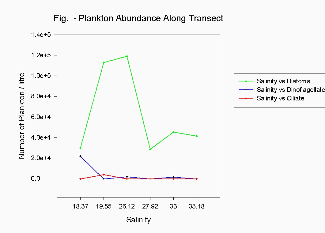
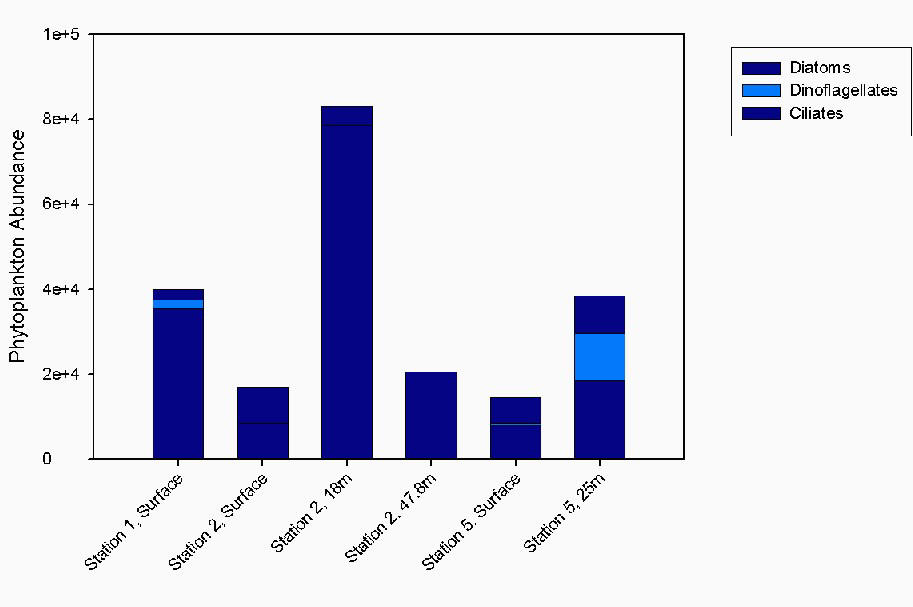
When looking at
the individual species of phytoplankton on figure 3.3.3
the difference in species can be noted.
Diatoms were the most dominant species, with dinoflagellates and
ciliates hardly fluctuating in comparison.
The silicon peaks with the phytoplankton, which indicates
biological removal of silicon in the estuary (see
section 3.2 chemistry).
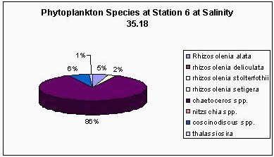
The most dominant species at either end of the transect is Chaetoceros
sp, although at station 6 near the breakwater, this constituted 86% of
the phytoplankton, whereas at station 2 it is only 31%
(see figure 3.3.5). This
diatom is probably responsible for most of the removal of silicon from
the estuary. |
|
||
|
Figure 3.3.3. A graph showing phytoplankton group abundance as recorded on 30/06/2005 in Tamar estuary. |
|||
|
|
|
||
| Figure
3.3.4
Phytoplankton species proportions at station 1, with a salinity of
18.37.
|
Figure 3.3.5. Phytoplankton species proportions at
station 6, with a salinity of 35.18, showing Chaetoceros as the
dominant species
|
||
|
|
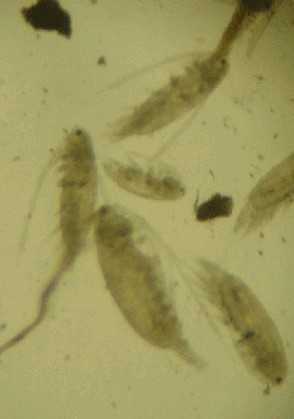
Diatoms were the most
abundant, followed by dinoflagellates and few ciliates were found in
the estuary, which may be due to grazing by zooplankton.
Ciliates are principally controlled by copepod grazing
(Rodriguez et al, 2000), in one sample 729 copepods were found in
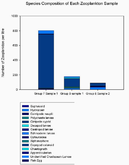
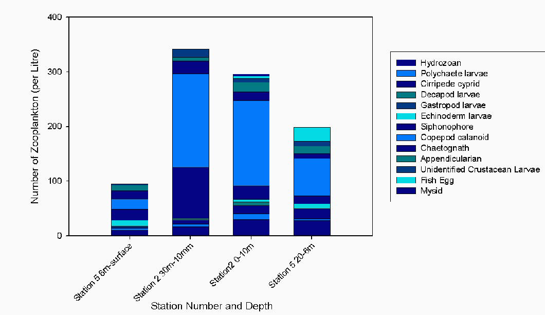
10ml, and no ciliates. Variations in copepod populations are typically controlled by the hydrodynamic characteristics of the water column. Some copepods are found throughout the year rather than only in peaks of nutrients, hence the vast amount of copepods found in most samples. Figure 3.3.9 show the most common species of zooplankton found. Many gelatinous siphonophores and hydrozoans were found nearer the mouth due to the lower motility compared to other zooplankton species. The breakwater acts as a barrier on the ebb tide hence trapping the zooplankton at the estuary mouth. |
||
|
|
|
||
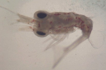
|
Figure 3.3.6. Example of a decapod at 30 magnification |
|||
 |
|||
|
Figure 3.3.7. Example of a copepod at 30 magnification |
Figure 3.3.8. Example of siphonophore (centre) and hydrozoa (left and right) at 30 magnification |
||
|
Figure 3.3.9. Species composition of zooplankton samples at 3 stations on 30/06/05. |
|||
Conclusion
The Tamar estuary is a partially mixed, salt wedge estuary, typical of those found in the south west of England (www.jncc.gov.uk/ProtectedSites/SACselection/habitat). Numerous small streams and discharges enter the estuary from the head to the Tamar Bridge which effects the biology, physics and chemistry of the water.
The estuary is strongly stratified at the head of the estuary where fluvial input is dominant, compared with the mouth of the estuary, where tidal and marine factors dominate. However increased water velocity at certain areas ie the Narrows, influence mixing within the estuary, changing the characteristics from partially mixed, to well mixed.
The estuary is heavily influenced by anthropogenic input as described in our chemical data. The estuary has shown to be a large sink for inorganic nutrients and an area of high biological productivity. Our results have shown that the Tamar estuary does act as a filter for terrestrial influxes into the open sea.
|
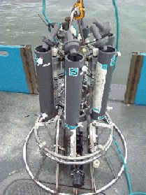
On the 10th July, 2005 the research vessel Bonito was used to survey the area of Hand Deeps. The site location was approx 16 miles to the south west of Plymouth (see Figure 4.1). The aim was to investigate the possibility of thermocline stratification of the water column offshore due to the dramatic change in weather conditions over the last few days. We also chose to investigate vertical mixing in the offshore waters and to observe the effect that Hand Deeps may have on this process. Vertical mixing has a profound influence on the physical and chemical properties of the surface layer of the ocean that in turn, largely controls the abundance and distribution of planktonic organisms (Kiorboe, 1993). The instruments used to investigate this were; CTD, fluorometer, transmissometer, secchi disk, zoo plankton net, and ADCP.
|
|
|
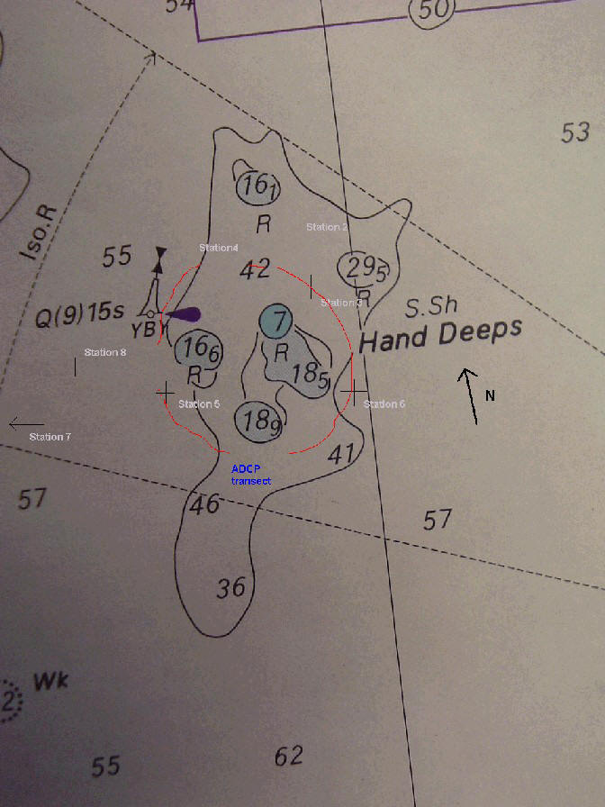
Background Seven stations were analysed during our survey day on the Bonito survey vessel. These were chosen to assess the mixing, in terms of geographical locations, around the Hands Deep. The survey stations are shown in the chart below (Figure 4.1). The weather forecast for the 10th July 2005 from the met office website was winds of 3-5 knots, with an atmospheric temperature of 24°C and a swell of about 2ft. The water temperature in Plymouth Sound had risen by an average of 3°C since the previous day (9th July, 2005). Weather on the days leading up to the investigation was also taken into consideration because of the effect it may have had on the thermal stratification of the water column. |
|
|
Figure 4.1. A chart showing the location of the survey points and ADCP transect around Hand Deeps |
|
| Referring to tidal diamond C
from the charts, it
was shown that at mid-day on 10th July 2005, the current was flowing on a bearing of
267°, at a speed of 1 knot. This is not the exact data for the surveying
area, but the most accurate data available. The tide time for the 10th
July for Devonport was:
|
|
| High Tide
08:00 4.95m 20:10 4.93m
Low Tide 14:10 1.38m |
|
| Data Analysis Station 1 |
Station 1 was positioned at the breakwater and was used for a shake-down, therefore data collected here has not been included in this report. |
| Station 2 |
|
|
|
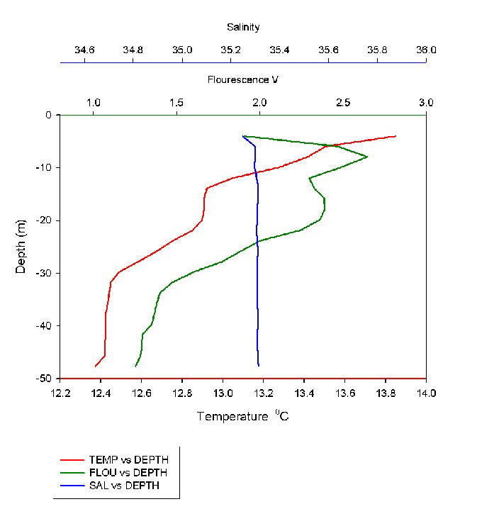
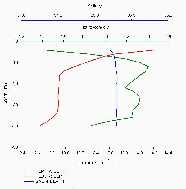
Figure 4.2 shows a vertical profile of salinity, fluorescence and temperature variation. The location of this station is 50 12.803 N -04 20.337 W. The temperature profile demonstrates a seasonal thermocline and the Richardson number of 1.12 for this station, suggests that the water column was stable and strongly stratified. The water was warmer in the first 15m of the water column, due to the increase in temperature over the previous 3 days, this correlates with the fluorescence peak at 10 metres depth, and the chlorophyll values also increased at this point. (Figure 4.13). The highest abundance of phytoplankton was also found at station 2 (Figure 4.7) at a depth of 18m, this corresponds to a high number of zooplankton also found here (at the trawl from 30m - 10m depth), which suggests that the zooplankton may have been grazing on the phytoplankton (Figure 4.6). Higher temperatures and upwelling may have been responsible for the surge at 10m depth. The temperature change of the water from 15m to 30m may have been due to a cold water upwelling from the recent bad weather and the mixing processes around Hand Deeps. The secchi disk depth (Figure 4.12) showed that the euphotic zone was at its shallowest at station 2 which correlates with the increase in SPM (suspended particulate matter) found in the water, suggesting high levels of plankton at this location. At the time of collection at this station, high numbers of zooplankton were visibly obvious and the specimens were much larger in size. The salinity remained almost constant throughout the vertical profile with no resounding features other than an initial lower reading that was generated by a bubble in the recording. The Oxygen concentration, nitrate and phosphate values confirm that the water column was stratified (Figure 4.8, 4.9, 4.11), with an obvious change at 18m, indicating a shallow euphotic zone at this location. The compensation depth was approximately 18m, below which the phytoplankton cease to utilize the nitrate and phosphate and only respiration occurs. Silicon concentration increased below the seasonal thermocline, the reduction above was due to the large number of diatoms utilizing the silicon for frustule formation (Figure 4.10).
|
|
Figure 4.2. Fluorescence, Salinity and Temperature at station 2 plotted verses depth. |
|
Station 4 Figure 4.3 shows a vertical profile of salinity, fluorescence and temperature variation. The location of this station was 50 12.728 N, -4 20.677 W. The temperature profile at station 4, in comparison to station 2, shows stronger mixing, shown in the graph by the increase in gradient and the reduction of a definite upwelling. The Richardson number concurs with this data, with a value of 0.64 which shows that the water column was less stable than at station 2, and hence more mixing occurred. The reason for this occurrence is the location of the site (Figure 4.1) being in the path of the current. The fluorescence shows a peak at depth of approximately 12 metres which may be due to the rock influencing the upwelling and mixing near the station. Unfortunately no samples were taken from this site due to time restriction which is why we can only hypothesize this situation. The secchi disk shows a larger euphotic zone as the depth of the disk is 2 metres greater than station 2, which indicates either less SPM in the water column, or that the SPM is lower down in the water column. The fact that the chlorophyll values peak at this depth suggests that the SPM is lower in the water column and that plankton make up the majority of the SPM. Again, salinity shows little variation offshore. |
|
|
Figure 4.3 Fluorescence, Salinity and Temperature at station 4 plotted verses depth.
|
| Station 5 | |
|
|
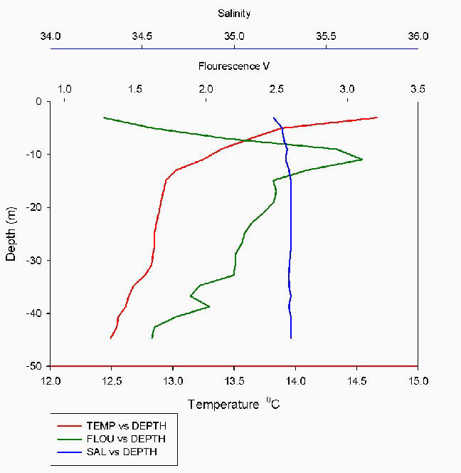
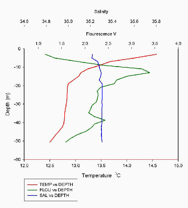
The location of Station 5 is 50 12.478 N, -4 20.643 W and this station appeared to be the most well-mixed of all stations. This is confirmed by the temperature gradient being more gradual than the previous station, no obvious stratification and a relatively low Richardson number (0.56) compared to the other stations in the survey. As observed at station four, the result of this is due to the site being positioned in the path of Hands deep (Figure 4.1). The fluorescence values also demonstrate the mixing profile of the water column, with a less pronounced spike at depth. The chlorophyll values were higher at Station 4 than those at Station 2 but showed little variation with depth (Figure 4.13). Figure 4.6 shows a more diverse phytoplankton population with less abundance than at Station 2. The euphotic zone was shallower here than at Station 4 but still greater than Station 2 (Figure 4.12). The continual gradient of oxygen concentration (Figure 4.8) confirms that the water column at this station was well mixed at the time of sampling. The chemical analysis, unlike station 2 showed no obvious stratification, as was the case for all nutrients. The silicon and nitrate concentration was much lower in this region than at the previous location, which may be because the upwelling was greater around this region therefore there would be an increase in nutrients in such a restricted zone (Figure 4.9 & 4.10). The increase in phosphate concentration shown in Figure 4.11 was caused by the reduced amount of plankton utilizing the phosphate. As with the silicon there was a restricted zone due to the increased upwelling. Salinity remained relatively constant due to the presence of a thermocline offshore, as opposed to the estuarine halocline.
|
|
Figure 4.4. Fluorescence, Salinity and Temperature at station 5 plotted verses depth.
|
|
Station 8 |
|
|
Figure 4.5 shows a vertical profile of salinity, fluorescence and temperature variation. The location of this station is 50 12.506N -4 21.483W. This location is approximately half a kilometre away from Hand Deeps (Figure 4.1), hence the temperature profile showing stratification due to the seasonal thermocline. The mixing influence of Hand Deeps rock is less pronounced than the other stations sampled, which concurs with the Richardson number of 0.82, suggesting a reduction in mixing. A spike in fluorescence occurs at 11 metres, with a secondary spike at 39 metres, however the second spike was due to a bubble in the recording equipment. Due to the reduced amounts of upwelling, the chlorophyll and nutrient levels were found at a lower level than previous stations (Figure 4.12, 4.9, 4.10, 4.11). Due to lack of plankton samples, the amount of nutrients cannot be justified by population demand. Through the analysis of oxygen concentration, it was observed that there was a reduced number of plankton in this locality (Figure 4.8), and also no upwelling. The chlorophyll shows a high amount of phytoplankton present at that station at the time of sampling (Figure 4.13). The secchi depth shows the euphotic zone is deeper than at Station 2, this is as a result of SPM found at depth due to decreased upwelling (Figure 4.12). |
|
|
Figure 4.5. Fluorescence, Salinity and Temperature at station 8 plotted verses depth. |
 |
|
|
|
Figure 4.6. The combined number of different species of zooplankton collected offshore on 10/07/2005 |
Figure 4.7. The combined number of different species of phytoplankton collected offshore on 10/07/2005 |
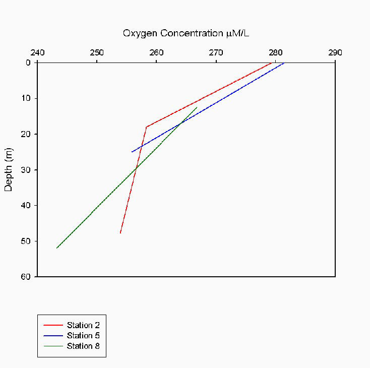
Figure 4.8. The oxygen concentration for stations two, five and eight. Samples were collected off shore on 10/07/2005 |
 |
 |
 |
|
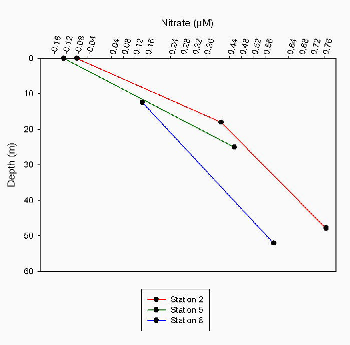
Figure 4.9. The nitrate concentration for stations two, five and eight. Samples were collected off shore on 10/07/2005 |
Figure 4.10 The silica concentration for stations two, five and eight. Samples were collected off shore on 10/07/2005 |
Figure 4.11. The phosphate concentration for stations two, five and eight. Samples were collected off shore on 10/07/2005 |
|
|
|
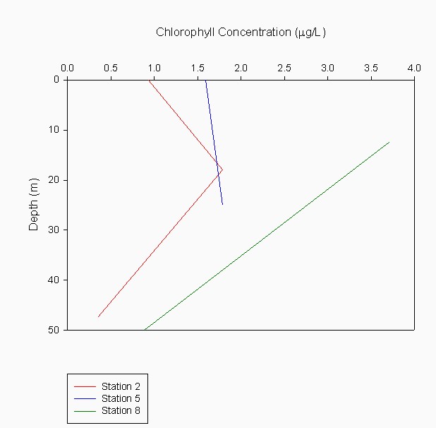
| Figure 4.12 secchi depth of all stations surveyed on 10/7/2005 | Figure 4.13 Chlorophyll concentration for stations two, five and eight. Samples were collected off shore on 10/07/2005 |
Offshore Overview and Conclusion
The offshore sites sampled on 10th July 2005 were discrete and therefore cannot be used to observe large scale processes. To gain a better overview of the effect of Hand Deeps, satellite data was analysed to compare the differences in sea surface temperature (SST) . The satellite referenced was AVHRR (Advanced Very High Resolution Radiometer) and was processed by the RSDAS (Remote Sensing Data Analysis Service) section of Plymouth Marine Laboratory. The SST data was collected using 6 different sensors that sample different wavelength bands and therefore forms a multi-spectral analysis for SST. The satellite used is a polar-orbiter and so passes over the site of Hand Deeps many times. However, due to the effect of the haze that formed during the day and cloud formation, some of the infrared radiation gets blocked out. Figure 4.12 was the only relevant image that could be obtained to show the temperature distribution on the sample day 10/07/05. It can be seen from this image that the region of water surrounding Hand Deeps Rocks is 2oC colder than the rest of the surrounding water. This is due to the rocks creating an upwelling region around them causing the surface water to be significantly cooler than the surrounding water body.
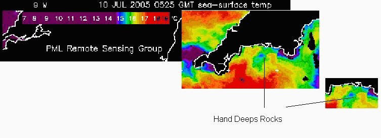 |
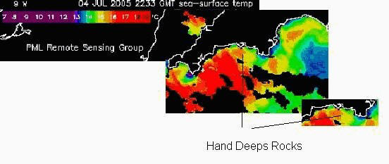
The observed upwelling Figure 4.12 of cooler water due to the current disturbance around Hand Deeps has only been observed when there has been calm sea conditions. This statement is based on the AVHRR data, comparing the fourth to the tenth of July. On the fourth the sea state was rough and the wind was 10-15 knots with gusts of 30 knots, (www.met-office.gov.uk), which greatly contrasts with the conditions on the 10th that were sea state flat/calm and a wind speed of 0-2 knots, which were measured in situ. |
|
Figure 4.12. A satellite SST imaging from a polar orbiting satellite on 10/07/2005
|
|
| Using this information and the
satellite data it is apparent that the mixing of the water column, due
to the wind and wave action, causes the upwelling water to be thoroughly
mixed with the surrounding surface water. This creates no observable
difference in the sea surface temperature Figure 4.13. However
when the sea state reduces significantly the surface water warms
considerably, this then allows the upwelling of cooler water from the
rocks, to be observed Figure 4.12. This is visible as the blue
pixels surrounded by the brighter colours, that indicate the warmer
waters. This correlates strongly with the in situ data that was
collected on the 10/07/05, onboard the research vessel Bonito.
To clarify further the hypothesis of the mixing and upwelling controls a circular transect around Hand Deeps was recorded with an ADCP (Acoustic Doppler Current Profiler) |
 |
|
Figure 4.13. A satellite SST imaging from a polar orbiting satellite on 04/07/2005 |
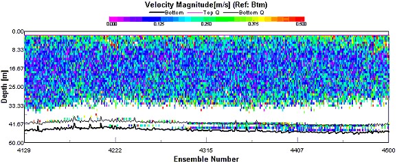 |
A transect was taken starting at 50°10.472N 4°20.330W, heading in a circular path around Hands Deep in a clockwise motion starting from the South East corner, hence the variation in velocity direction from initially 0 degrees to 180 degrees from when the Bonito had changed its bearing for the eastern side. Velocity magnitude remains even around the rock, with velocity averaging 0.125 m/s between 9 and 30 m depth, becoming greater nearer the surface getting upwards of 0.250 m/s. Backscatter shows a peak at around 10 m depth, indicating zooplankton just above the thermocline grazing upon the phytoplankton in this area, which is also shown from the data collected by CTD at station 4 and station 2. To clarify the station data collect from locality 7 and 8 a transect west of Hand Deeps was recorded with an ADCP. |
|
Figure 4.14. Velocity magnitude for the circular transect around Hand Deeps on 10/07/2005 |
|
|
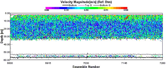
This transect was taken to the west of Hand Deeps, following where the current flows from east to west at the time of day as tide was slack. Starting at 50°12.449N 4°22.048W and finishing at 50°12.477N 4°22.227W. Current velocity magnitudes are greater here than at Hand Deeps, the top 10 m magnitude averages are above 0.30 m/s, heading South West. Deeper currents were found between 10 and 30 m depth were heading in a more westerly direction averaging at above 0.130 m/s. Backscatter peaks between 10 and 20 meters depth, which matches with the fluorescence peak found at station 8 as shown on the thermocline, indicating zooplankton grazing upon a phytoplankton bloom which would be at this point. This concurs with our CTD data of this surveying area. |
 |
|
Figure 4.15. Velocity magnitude transect west of Hand Deeps on 10/07/2005. |
The main control on our survey area, Hand Deeps, is physical processes these in turn influence the chemical and biology. This is proven from the CTD profile from each station. Where the stations that were located in the shadow of the Hand Deeps rock show a greater physical mixing thus changing the biological and chemical components. Upwelling has a strong contribution to the physical attributes shown, upwelling also influences the abundance of nutrients thus enhancing the primary production.
Although Hand Deeps has a significant impact on the ocean constituents it is only influential to the immediate surrounding waters. This is proven from the data collected at station eight where the water column more typical oceanic model. Therefore the influence of Hand Deeps on estuarine water will be little to none.
Grasshoff K, Kremling K & Ehrhardt M (1999). Methods of seawater analysis. 3rd ed. Wiley-VCH
Johnson K & Petty RL (1983). Determination of nitrate and nitrite in seawater by flow injection analysis. Limnology and Oceanography, 28: 1260-1266.
Morris A. W. A.J. Bale and R. J. M. Howland (1981). Chemical Variability in the Tamar Estuary, South-west England. Estuarine, Coastal and Shelf Science (1982), 14: 649-661
Morris AW, Bale AJ & Howland RJM (1981). Nutrient Distributions in an Estuary: Evidence of Chemical Precipitation of Dissolved Silicate and Phosphate. Estuarine, Coastal and Shelf Science, 12: 205-216
Parsons T R, Maita Y & Lalli C (1984). A manual of chemical and biological methods for seawater analysis. 173p. Pergamon
Rodriguez F, Fernandez E, Head RN, Harbour DS, Bratbak G, Heldal M, Harris RP (2000) Temporal variability of viruses, bacteria, phytoplankton and zooplankton in the western English Channel off Plymouth. Journal of Marine Biological Association, 80: pp.575-586
Tattersall, G.R., Elliot, A.J. and Lynn, N.M.(2003) Suspended sediment concentrations in the Tamar Estuary. Estuarine, Coastal and Shelf Science, 57: 679-688
Uncles, R.J., Elliott, R.C.A and Weston, S.A.(1985) Observed Fluxes of Water, Salt and Suspended Sediment in a Partly Mixed Estuary. Estuarine, Coastal and Shelf Science, 20:147-167
Web References
www.jncc.gov.uk/ProtectedSites/SACselection/habitat. accessed 12/07/2005.
www.npm.ac.uk, accessed 10/07/2005
www.met-office.gov.uk. accessed 12/07/2005.