Plymouth Field Course 2005
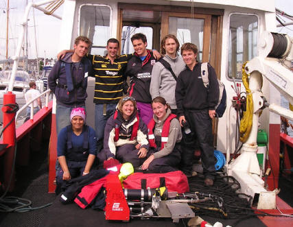
Group 6
Iain Dickson, Jeff Eliot, Andy Bruce, Ignacio Pagnola Schiavon, David Leonard, Siddhi Joshi, Michelle Fox, Anna Macey.
![]()
![]()
![]()
![]()
Between 30th June -13th July 2005 a group of 8 intrepid oceanographers from Southampton University undertook the challenge of producing a scientific breakdown of the biological, chemical and physical properties of the estuarine, coastal and offshore environments that run alongside, and surround the city of Plymouth. To further this intense investigation, an attempt was also made to link these properties to the geology of the area, using a plethora of geophysical and field surveys.
The Tamar estuary (the focus for study of the estuarine section of the investigation) is a Ria (drowned river valley) that was partially flooded during the Flandrian transgression of the last 10,000 years. It is comprised of the rivers Tamar, Lyner and Tavy and is a macrotidal estuary (mean neap and spring tidal ranges of 2.2 and 4.7m respectively) with semidiurnal and flood dominant characteristics. These influence it to being a partially mixed estuary (Dyer, 1997).
To collect the data for the investigation a range of vessels were used to survey the different sections of the waters around Plymouth:
The investigation, however, was not only an exercise for practical data collection and analysis but one of teamwork. During the 2 weeks, the group had to work together on the boats to make sure all the necessary data for the investigation was collected, then in the labs to be able to analyse and select the appropriate data for the final report. Without this work ethic, the sheer volume of data could not have been analysed and the integrity and structure of the investigation would have been compromised.
Throughout this website click on thumbnails to enlarge.
| Date | Survey Vessel | Location | Tides | Weather | Sampling |
| 30th June 2005 | Natwest II |
Grid - Cawsand Bay Transect - In front of Breakwater at 50°20.236'N, 4°11.34'W & 50°19.75'N, 4°11.75'W |
HW - 12:30 GMT (4.59m)
LW - 18:50 GMT (1.88m) |
Cloud cover - 8/8 Wind - Force 4-5 W Heavy showers, brightening up in the afternoon |
Side scan sonar,
Van Veen grab |
Figure 1. Natwest II |
Originally, the group intended to survey a couple of wrecks just outside Plymouth Sound, however due to rough weather conditions (force 4 – 5 South Westerlies) it was decided that the survey of these wrecks would be highly impractical, inaccurate and potentially hazardous to the crew. A safer survey site was chosen in Cawsands Bay, which offered shelter from the wind.
An initial transect line was constructed between 50°20.236'N, 4°11.34'W and 50°19.75' N, 4°11.75'W. Using the onboard computer systems a grid of 4 more parallel lines was generated. The swath of the side scan sonar was a total of 150m, 75m each side of the vessel. The grid lines were spaced 100m apart in order to attain an overlap of the data recorded. This ensured that the area under investigation was completely covered within the survey providing a detailed picture of the sea bed.
 Figure
2. The 'fish' used onboard Natwest II.
Figure
2. The 'fish' used onboard Natwest II. |
Using GPS for navigation the Natwest II moved along the grid lines at a speed of roughly 4 knots, towing behind it the transmitter and receiver for the side scan sonar system which is also known as a “fish” (figure 2). This sends out an acoustic pulse which is reflected off the sea bed or any items in the water column, back to the fish as backscatter. This then sends the data to a computer onboard which continuously logs the data onto a roll of paper, known as the trace. This was then interpreted to obtain a map of the surveyed grid and transect.
The side scan sonar system however operates on a set of assumptions:
 Figure
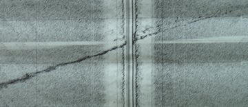
3. Wake of boat on trace.
Figure
3. Wake of boat on trace. |
The fish can pick up artefacts and distortions, which will be recorded. An artefact is defined as “an apparent feature that appears on the trace, which does not represent any actual solid feature on the seabed” (Blondel & Murton 1997). For example this could be created by crossing the path of a wake left from another vessel. This occurred during our survey of Cawsand Bay and can be seen as a darker diagonal line, which runs across our trace (figure 3). Distortions of the data occur when the actual shape of a physical feature on the sea bed (after the normal correction) is changed. This normally occurs if the fish rolls in the water or the seabed slopes away underneath the vessel.
After the initial grid was completed, a longer transect was constructed from 50°20.079'N, 4°1.226'W to 50°19.840'N, 4°8.006'W which stretched from Cawsand Bay across Plymouth harbour, running parallel in front of the breakwater. For this part of the survey the frequency of the GeoAcoustic side scan system was changed from 100KHz to 500kHz (AST time: 10.47.03 GMT) This resulted in a more suitable resolution for the changing seafloor topography. Mid-survey however, some Navy destroyers and frigates were entering the harbour and so temporarily the survey along the transect had to be suspended until the ships had passed. To make best use of the delay, the group then decided to extend the original grid by running two more parallel lines in the same fashion as before on the edge furthest from the shore starting at 50°20.2'N, 4°11.1'W. Once the Navy vessels had passed the transect running in front of the breakwater was completed.
 Figure
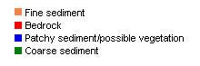
4b. Bedrock
Figure
4b. Bedrock |
 Figure
4a. Fine sediment
Figure
4a. Fine sediment |
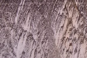
The map (figure 5) produced from the side scan sonar trace shows areas of fine sediment (figure 4a), bedrock (figure 4b), coarse sediment and also patchy material which could include boulders, pebbles and possibly seaweed. The majority of the survey area was found to be composed of fine sediments. This is supported by grab and dredge samples. These samples were taken using a Van Veen grab and a pipe dredge. The location and descriptions of the sediment (both the biogenic and minerogenic factors) and the species recovered from the samples are described below.
From studying charts of the area, for example, it is noticeable that there is an outcrop of rock from the land at 50°20.20'N, 4°11.35'W (244000E, 51000N). This lies close to the seabed areas that we have suggested are bedrock and therefore probably indicates an extension of the land-based geology.
The transect data was processed by performing along track corrections, with respect to the ship’s velocity, and across track corrections, by mainly correcting for the water column. Areas of fine sands, coarse sands and bedrock were found. Regular symmetrical ripples were found in the coarse sands, possibly due the breakwater altering the water current strength and direction. A patch of fine sand was found amongst the bedrock, as indicated by low energy reflections found within the bedrock shadow zones. Dip layers and faults were also visible on the bedrock. The transect further indicated that the land based geology extended underwater.
· Sample 1. Grab sample (figure 6), (50°19.64'N, 4°11.43'W): Grain sizes in this sample are between 0.1 mm and 1mm (very fine and coarse sand respectively). Biogenic particles, including shells of microscopic organisms are present, as are fragments of larger shells. This is the most unsorted of the various samples taken. Approximate composition includes quartz, feldspar and sheet silicates such as mica. These probably originate from granites around Dartmoor that have been eroded by the Tamar River in its upper reaches and transported to the study site.
Sample 2. Pipe dredge 1 (figure 7), (50°19.64'N, 4°11.57'W): The average grain size within this sample is approximately 0.5 mm i.e. fine sand. This sample is well sorted, consisting of mostly minerogenic, homogenous material. It includes similar minerals to those from the grab sample but does not contain shell fragments.
Sample 3: Pipe dredge 2 (figure 8) (Start - 50°19.6'N, 4°11.6'W, End - 50°19.7'N, 4°11.5'W): The grain sizes of this sample are approximately 0.1 mm, which corresponds to very fine sand. The particles are almost entirely minerogenic.
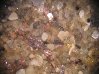 Figure 6. Grab sample
 |
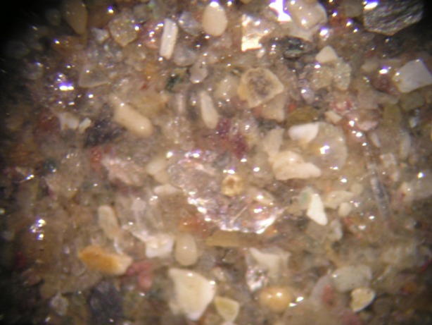 Figure 7. Pipe dredge 1
 |
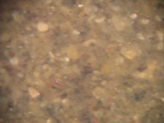 Figure
8. Pipe dredge 2
Figure
8. Pipe dredge 2 |
· Grab 2: (50°19.64'N, 4°11.43'W). Various Polychaetes, Crustacea (e.g hermit crab) and Bivalves (e.g clam) were found in this grab sample.
· Pipe dredge 2: (Start - 50°19.6'N, 4°11.6'W, End - 50°19.7'N, 4°11.5'W). Juvenile razor clams and a Netted Whelk were among bivalves that were found in this pipe dredge. Also found was a Brittle star (figure 11 )
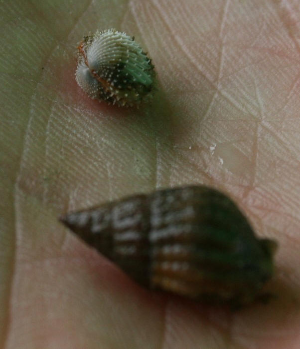 Figure
9. Netted and Spiny Cockle
Figure
9. Netted and Spiny Cockle |
 Figure 11. Brittle
star, juvenile mussel and a small clam.
Figure 11. Brittle
star, juvenile mussel and a small clam. |
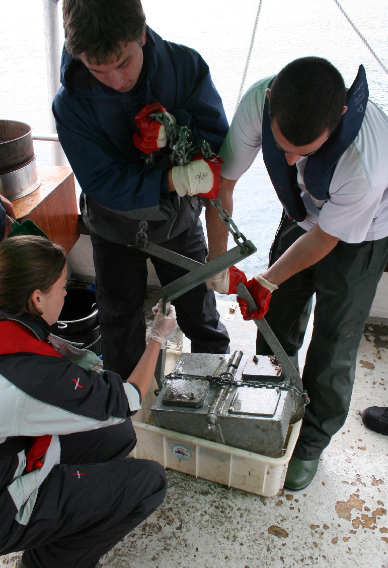 Figure
10. Van Veen grab.
Figure
10. Van Veen grab. |
| 3rd July 2005 | 10th July 2005 |
| Date | Survey Vessel | Location | Tides | Weather | Sampling |
| 3rd July 2005 | Bill Conway | As seen on Figure.... |
HW - 1530 GMT (4.57m) LW - 0920 GMT (1.89m) |
Cloud cover - 3-5/8 Wind - SW veering W force 3-4 Bright and sunny with slight cloud cover |
CTD rosette, ADCP, Plankton net, Water samples, |
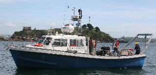 The
Bill Conway (length 11.7m) is a coastal vessel designed for scientific research.
It was used to survey the Tamar estuary from the Plymouth breakwater up the
estuary to the Tamar bridge (see map). The Bill Conway is equipped with
ADCP, a CTD complete with
rosette sampler, fluorometer and transmissometer, GPS and logging computers. The data collected from the Bill
Conway was compiled with data collected from further up the estuary by the group
5 on the same day using RIBS (Rigid inflatable boats). This allowed for a
view of the whole estuary across its salinity range. The aims of
this investigation were: to construct estuarine mixing diagrams for phosphate,
nitrate and silicate; compare plankton populations from different areas of the
estuary; and to investigate and outline the physical properties of the estuary.
The
Bill Conway (length 11.7m) is a coastal vessel designed for scientific research.
It was used to survey the Tamar estuary from the Plymouth breakwater up the
estuary to the Tamar bridge (see map). The Bill Conway is equipped with
ADCP, a CTD complete with
rosette sampler, fluorometer and transmissometer, GPS and logging computers. The data collected from the Bill
Conway was compiled with data collected from further up the estuary by the group
5 on the same day using RIBS (Rigid inflatable boats). This allowed for a
view of the whole estuary across its salinity range. The aims of
this investigation were: to construct estuarine mixing diagrams for phosphate,
nitrate and silicate; compare plankton populations from different areas of the
estuary; and to investigate and outline the physical properties of the estuary.
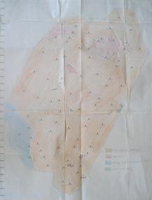
Sampling was carried out starting from the Tamar Bridge, moving down river to Plymouth breakwater against a flood tide. Locations for sampling were decided upon by their importance as either a confluence of rivers or as being ideal locations for studying the key flow patterns of the estuary. Sampling locations can be seen on the map (figure 12). At each station, typically a CTD profile and an ADCP transect were carried out, but at some stations further sampling was taken including: sub-surface water samples, taken using the rosette sampler on the CTD (subject to the profile of the water column); zooplankton trawls using a 200µm plankton net; surface phytoplankton samples taken using a bucket; and secchi depth measurements. The table below summarizes which measurements were taken at which station.
|
Station Number |
Measurements Taken |
|
1 |
T, CTD, SD, 3 x WS, Z, P |
|
2 |
T, CTD, SD, 2 x WS, P |
|
3 |
2 x T, CTD, SD, WS |
|
4 |
T, CTD, SD |
|
5 |
T, CTD, SD, 2 x WS |
|
6 |
T, CTD, SD, WS |
|
7 |
T, CTD, SD, 2 x WS, P |
|
8 |
CTD, SD, P, Z |
|
9 |
T, CTD, SD, 3 x WS, |
|
10 |
CTD, SD |
Key - T – ADCP transect, CTD – CTD profile, SD- secchi depth, WS – water sample, P – Phytoplankton sample, Z – Zooplankton trawl.
 Figure
13. Water sampling
Figure
13. Water sampling |
 Figure 15. Secchi manager Jeff, pre-deployment
 |
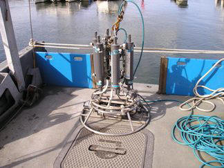 Figure 14. CTD
|
Estuarine mixing diagrams were plotted for nitrate, phosphate and silicon, with salinity as an indicator of conservative mixing. The Bill Conway CTD and the TS probe from the RIBs were used to examine the same water mass, at the same depth. The difference between the two salinity readings was 0.01. Group 5's Ribs data was therefore adjusted to match with the CTD data. The Theoretical Dilution (TDL) line was also plotted, linking the riverine and the marine end members. This line was also extended to estimate the concentration at 0 salinity. All three nutrients are riverine constituents, with higher concentrations in river water than in seawater. Assumptions of this one dimensional mixing model include:
The system is in steady state with constant end member concentrations on time scales greater than the residence times of the estuary.
There is only one riverine and marine end member. It is important to note that the Tamar estuary has the River Tamar, the River Tavy and the Lynher River entering up the estuary.
It is assumed that there are not any additional sources of dissolved material external to the water column; e.g. from sediment pore waters.
 Figure
16. Nitrate mixing diagram
Figure
16. Nitrate mixing diagram |
In the nitrate estuarine mixing diagram (figure 16), the points are found on the line suggesting conservative mixing. After examining previous data, two anomalies have been suspected, including the riverine end member of 275 µML and the 373µML. Nitrate is not only a key nutrient for photosynthesis, but also for the anoxic organic matter decay process.
 Figure 17. Phosphate mixing diagram
 |
The phosphate profile (figure 17) shows there is non conservative mixing occurring, with removal at low salinities in the lower estuary and addition in the upper estuary. Anthropogenic inputs as a result of sewage, agriculture and urban runoffs near Devonport may be responsible for the addition. Removal is likely to be occurring due to a combination of factors, including uptake by phytoplankton. Dissolved Inorganic Phosphate (DIP) and Dissolved Organic Phosphates (DOP) are used for producing high energy compounds such as ATP and genetic material, as well as phospholipids in the cell membrane.
The Redfield Ratio states that the relationships between the concentrations of nutrients, in the marine open ocean, with the Carbon: Nitrate: Phosphorus: Oxygen ratio being 106:16:1:138 (Redfield, 1958). In this case however, the N:P ratio observed, in a contrasting estuarine environment, does not follow the Redfield ratio. The N:P ratio in the riverine end member concentrations has been found to be more like 88:1, (155:1.75) rather than 16:1. This deviation from the Redfield ratio suggests that there are additional factors controlling the nutrient concentrations of the Tamar estuary. Inputs of agricultural nutrients as well as the precipitation in the estuary may be key factors in determining estuarine nutrient concentrations. Seasonal changes in the rainfall and agricultural inputs can be examined to extend the investigation. Hence, it is important to note that estuaries are constantly in transition, being dynamic environments, with a constantly changing chemistry.
Figure 18 shows that all the points are found below the TDL, indicating non conservative mixing, with net removal from the estuary. The irregular distribution of the points below the TDL indicates a non uniform removal of silicon from different parts of the estuary. A possible explanation for this removal may be due to uptake of silicic acid by diatoms and other silicon utilizing phytoplankton, to form the diatom frustules.
H4SiO4 (aq) à SiO2 – nH 2O (s)
 Figure 18. Silicon mixing diagram.
 |
Hence, an increased amount of silicon is removed in areas with a high diatom population, where there is high primary productivity. This pattern of primary production along the estuary is shown in the phytoplankton counts, with the population dominated by diatom species. Therefore, physical factors affecting primary production, such as light, turbidity and the mixed layer depth may influence the uptake of silicon and hence the silicon concentrations in the estuary. As there are seasonal changes in the primary production, silicon only exhibits non conservative behaviour during the summer months. Another possibility as suggested by Morris et. al. 1981 , is that the removal may be due to non biological factors, such as “tidally induced re-suspension and sediment deposition.”
 Figure
19. Chlorophyll a mixing diagram
Figure
19. Chlorophyll a mixing diagram |
A mixing diagram (figure 19) has also been plotted for the chlorophyll a concentration to show how the levels of primary production change throughout the estuary. The chlorophyll a concentration generally decreases with increasing salinity. This may be due to changing physical factors in the upper estuary.
 Figure 20. Chlorophyll a
against oxygen.
Figure 20. Chlorophyll a
against oxygen. |
The dissolved oxygen concentration is also dependent on photosynthesis, as oxygen is produced during photosynthesis. A graph showing the oxygen concentration against the chlorophyll concentration shows a positive correlation for stations down the estuary (Figure 20). In the upper estuary (Stations 6, 7 and 9) an area of low chlorophyll, high oxygen is observed. This may be due to an additional source of oxygen to the estuary, due to increased mixing and turbulence as it is in a more exposed area.
Surface phytoplankton samples were taken at 9 different stations, 5 by the RIB group upstream and 4 by the Bill Conway group in the lower part of the Tamar Estuary. At all the stations, except one, diatoms were the most abundant phytoplankton taxa. The exception was at station 9, which had the lowest salinity of all the phytoplankton samples taken. Dinoflagellates were present at three of the stations, however they were present in very low abundances and therefore this cannot be seen in figure 22. The sample from station 9 was dominated by ciliates. At this point in the river the water depth was at its shallowest and therefore a surface sample probably contained suspended benthic ciliates.
|
|
|
 |
 Ceratium furca Ceratium furca |
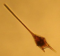
Figure 21. Phytoplankton found in samples
|
|
 Figure
23. Chlorophyll a mixing diagram.
Figure
23. Chlorophyll a mixing diagram. |
From figure 22 it can be seen that there is a general decrease in phytoplankton abundance as distance is moved down river and out into the estuary. There is an exception to this at station 14, where there is a decrease in abundance to ~6x10⁴ cells L-1, and then an increase at station 16. This decrease however in terms of phytoplankton abundance is actually a very small difference and thus we can therefore conclude that there is a trend of decreasing abundance with increasing salinity. At the head of the river nutrient levels are high due to anthropogenic influences and agricultural run-off from land. As you move towards the mouth of the river and into the estuary, nutrient levels decrease due to utilization by phytoplankton and other organisms. Thus the decreasing abundances of phytoplankton could be due to nutrient limitation at higher salinities.
Chlorophyll a is used as an indicator of phytoplankton abundance. There is a slight negative correlation of decreasing chlorophyll a with increasing salinity (figure 23), which corresponds with the phytoplankton results.
The estuarine zooplankton was collected from Bill Conway and on one of RIBs. The samples were collected using two different methods. On the Bill Conway the same method was used as on Bonito (see method), and two stations were sampled. The first upstream at station 1 (50°24.587'N, 4°12.189'W) where salinity varied from 24.2 at the surface to 31.7 near the river bed. The second sample was taken from station 8 (50°20.579'N, 4°08.685'W), by the breakwater where salinity stayed between 34 – 35 throughout the water column.
On the RIB, the method used to retrieve data was slightly different. The boat anchored up and the zooplankton net was lowered downstream for five minutes to collect the sample at 50°26.730'N, 04°12.311'W, the salinity at this station was 26. A flow meter at the mouth of the net was used to determine the volume of water sampled. Once the net has been retrieved it was washed down to ensure all samples were in the sample jar then formalin was added to preserve the sample.
In the sample taken on the RIB (salinity 26), Copepods made up 72% of the total sample, Decapod larvae made up 13% (figure 24). Copepods were also most dominant at station 1 (see map) from Bill Conway where they made up 46% of the total sample. Decapod larvae were again the second most abundant making up 21% of sample taken. This suggests that the distribution of Decapods is not dependant on salinity since they are found in significant numbers in both the estuarine system and offshore. Decapod larvae however make up a larger percentage of the zooplankton community in the estuary than offshore. This would suggest that the estuary is a more suitable location for the larvae to develop.
The final zooplankton sample was taken at station eight, just inshore of the breakwater where the salinity rises up to 34+. There is then a big change in what types of zooplankton dominate the samples (figure 25). The most common zooplankton from this sample are Hydrozoans making up 47% of the total sample. There are ten different species that make up the sample indicating a higher diversity in the more saline water than in the fresher water (only 6 different species). Chaetognaths made up 12% of the sample, coupled with the high abundance of hydrozoans, this suggests that zooplankton distribution is more dependant on salinity than temperature differences along the estuary.
One of the limitations to the data recorded for estuarine zooplankton is that the samples taken and analysed were very small. As a result there is a danger of not collecting a sample that is representative of the community.
It was found that the estuarine communities of zooplankton were influenced to a greater extent by salinity variance throughout the estuary as opposed to temperature difference within the water column. This is however not the case for offshore zooplankton data (see offshore zooplankton conclusion).
At this most up-estuary station, transmittance (figure 26) increases with depth from 0.64 at 0.5m to 1.151 at 4.7m. It then decreases slightly back to 1.046 at 9.5m. Fluorescence (figure 26) shows a slight increase from 2.082 to 2.168 at 2.1m, before decreasing to 1.879 at 5.5m. It stays roughly constant to 8m then decreases again to 1.789 at 9.5m.
The temperature and salinity plot (figure 27) for this station displays a steady increase in salinity with depth from 23.1 to 30.2 at 4.2m. It then remains more or less constant with only a slight increase of 1.8 over the remaining 5.3m. The temperature profile, meanwhile, shows a strong thermocline from 2-4m.
Transmittance (figure 28) at this station steadily increases with depth from 1.3 at 0.5m to 1.62 at 12.5m then remains fairly constant with an increase of only 0.1m over the last 9m. Fluorescence (figure 28) shows a rapid increase from 1.53 at 0.7m to 1.93 at 4.3m. It then steadily decreases to a minimum of 1.5 at 21.7m.
The salinity profile (figure 29) at this station shows a steady increase with depth from 31.8 at the surface to 33.9 at 22.1m. Temperature (figure 29) readings display an abrupt decrease in the upper 2m of the water column. Below this, temperatures are steady.
At this station in the lower estuary, transmittance (figure 30) slightly increases from 1.84 at 0.9m to 1.91 at 4.5m. It then remains fairly steady, increasing to only 1.92 at 11.1m. In contrast to station 4, fluorescence (figure 30) at this station shows a large decrease over the upper 1.7m, from 1.612 to 1.17. It then gradually increases to a maximum of 1.92 at 10m.
The salinity plot (figure 31) for this station shows a slight increase with depth from 34.7 at 2.7m to 35.1 at 5.1m. It then remains approximately constant to the deepest reading, at 11.1m. The temperature profile (figure 31) at this station displays a prominent thermocline between about 2-4m, where the temperature falls by about 1°C.
Transect description:
| Time (GMT) | Latitude | Longitude | |
| Start of Transect | 08:55 | 50o24.5935'N | 4o12.1856'W |
| End of Transect | 08:56 | 50o24.6219'N | 4o12.1856'W |
Tidal state: Low Water: 0920 GMT. High water: 1530 GMT. The transect was measured during an ebb tide.
The first transect taken at station one demonstrates a surface layer movement, which is evidence of mixing most likely caused by wind. Pronounced bottom layer movement also indicates deep mixing in the water column.
The average backscatter plot (figure 32) shows high acoustic backscatter between 5-7m, which suggests the presence of zooplankton (and probably phytoplankton). The Richardson number (Ri) plot (figure 33) shows shear instability almost at every depth in the transect except at 1.9m depth where the Ri is clearly higher indicating the presence of a thermocline. If one examines the CTD data, there is clear evidence of a thermocline at this station between 2-4m, which can be seen in figure 27.
Transect description:
| Time (GMT) | Latitude | Longitude | |
| Start of Transect | 10:00 | 50o24.8721'N | 4o12.2894'W |
| End of Transect | 10:07 | 50o23.9544'N | 4o12.3697'W |
Tidal state: Low Water: 09:20 GMT. High water: 15:30 GMT. The transect was measured during a flood tide.
The backscatter contour plot (figure 34) indicates noise data near the bottom of the estuary on the side closet to the river Lynher. One plausible explanation for this is the scouring of the sea bed by strong tidal currents (velocity magnitude plot (figure 35) shows that the speed of the current is highest in this section of the transect also). The flow coming from the River Lynher mixing with that of the Tamar will also cause turbulence and in turn disturbance of the sediments. Ri numbers plot backs up this theory showing that there is instability and turbulent mixing (and therefore eddying) with values of less than 0.25 at these depths in the water column.
Transect description:
| Time (GMT) | Latitude | Longitude | |
| Start of Transect | 13:30 | 50o20.0534'N | 4o08.1624'W |
| End of Transect | 13:34 | 50o20.1775'N | 4o07.8927'W |
Tidal state: Low Water: 09:20 GMT. High water: 15:30 GMT. The transect was measured during flood tide.
The velocity magnitudes for this transect are higher at the surface than at the bottom. The highest velocities are found in the middle of the transect. There is a notable area next to the breakwater where the water is moving considerably slower than the rest of the channel. This is shown by a bluey/purple area on the left hand side of the diagram (figure 36). The high velocities are due to the narrow opening at the mouth of the estuary exposed to the coastal waters. There is noticeable backscatter (figure 37) near the surface (around 5m), probably due to the presence of zooplankton. The Ri number plot (figure 38) indicates extensive mixing throughout the water column since all the values are below 0.25.
 Figure
36. Velocity magnitude plot for station 9, transect 9.
Figure
36. Velocity magnitude plot for station 9, transect 9. |
 Figure
38. Richardson number plot against depth for station 9, transect 9.
Figure
38. Richardson number plot against depth for station 9, transect 9. |
Figure
37. Average backscatter plot for station 9, transect 9. |
| Date | Survey Vessel | Tides | Weather | Sampling |
| 10th July 2005 | RIBs |
HW - 07:56 GMT (4.7m) LW - 14.04 GMT (1.5m) |
Cloud cover - 1/8 Sunny and hot |
Water sampling, T/S probe, Plankton. |
In order to extend the estuarine investigation to lower salinities the use of RIBs was required. Since it is a macrotidal estuary the depths of the estuary at lower salinities were very shallow. The draught of Bill Conway was too great to reach these lower salinities whereas that of the RIBS was not. The main purpose of this part of the estuarine investigation was to attain a direct comparison of nutrient data with that collected on the day of Bill Conway practical.
The first sampling station was at the most up-river point accessible by RIB, near to the town of Calstock. To ensure that there was enough water to accommodate the draught of the boats a secondary port calculation was required to compensate for the distance up the estuary. The tide times mentioned above are those from the original tide tables. Moving down river, stations were then located at salinity intervals of approximately 2. These locations are shown on the map above (map). At each of these stations, readings were taken for water temperature, salinity, depth, pH, and oxygen concentration and saturation. The Secchi disc depth was also assessed and samples were taken for silicon and nutrients. In addition, oxygen samples were taken at 3 stations, using a Niskin bottle triggered just below the surface. With respect to the biological characteristics of the upper estuary, samples were taken for phytoplankton populations at 4 of the stations and a single zooplankton trawl was carried out at station 12.
As with the data obtained on the 3rd of July (when we were on the Bill Conway), analysis of the nutrient characteristics was undertaken, including the production of estuarine mixing diagrams for nitrate, phosphate, silicon, oxygen and chlorophyll. With the exception of silicon, these diagrams are not significantly different to the previous ones, shown above. In the case of silicon, it appears that a change has occurred in the removal processes over the time period between the samples (1 week). The pattern of removal seen on the 3rd of July (figure 39), as discussed above, is very irregular along the length of the estuary. The silicon plot for the 10th of July (figure 40), on the other hand, shows a smooth curve indicating similar removal rates along the entire length of the estuary and greater overall removal. This is most likely due to increased uptake by diatoms, which could have bloomed in the intervening week. This hypothesis is supported by the differing populations of diatoms found in the phytoplankton samples on each of these days. At the station with a salinity of 14, the total number of diatoms collected on the 3rd of July was 63,750, whereas on the 10th of July 141,000 were obtained. This corresponds with the fall in silicon concentrations seen over the time period.
| Date | Survey Vessel | Tides | Weather | Sampling |
| 7th July 2005 | Bonito |
HW - 0610 GMT (4.89m) LW - 1220 GMT (1.42m) HW - 1830 GMT (4.93m) |
Cloud cover - 7/8 Morning - 4/8
Afternoon. Wind - NW veering to W, force 4-5. Cloudy start, sun breaking through in the afternoon |
CTD, Mini-bat, Zooplankton, Phytoplankton and water samples. |
Offshore sampling was carried out on board a 15 metre vessel called the Bonito with the aim of investigating the effects of the Eddystone Rocks on the physical, chemical and biological properties of the offshore water column. Eddystone Rocks are located approximately 10 nautical miles off the coast of Plymouth. Because of its position in relatively deep waters it provides an interesting area to study in terms of the mixing processes and the effects of physical structures within the water.
Four stations were sampled during the course of the day. The first station (see map) was inside the breakwater on the west point. Station 2 (50°11.881'N, 4°14.827'W) and 3 (50°10.847'N, 4°15.430'W) were located around Eddystone Rocks. Unfortunately we were unable to sample enough stations around Eddystone due to the rough conditions of the sea, so the fourth station sampled was at L4 (50°15.020'N, 4°14.050'W). All station locations are marked on the map in figure 41.
At each station a CTD drop was carried out with chemical and biological samples acquired using niskin bottles mounted on the rosette sampler. The depths at which these samples were collected from were decided upon using the CTD profile of the water column. The samples were analysed for silicate, nitrate, phosphate, oxygen and chlorophyll a concentrations. Phytoplankton samples were also taken from the niskin bottles and stored in lugols. Zooplankton samples were collected using a 200µm plankton net. The net could be closed at depth using messengers allowing samples to be taken at various depths. The samples were preserved in formalin after collection. ADCP data was also collected for each station.
As well as the CTD and ADCP, the Bonito had a minibat. This is a towed CTD profiler with the ability to move up and down through the water column, continually collecting data. As well as the CTD, the minibat also had attached a fluorometer, transmissometer and a licor. The minibat was deployed at Eddystone and towed around the island. The path of the minibat can be seen on the map.
Nitrate, Silicon and Chlorophyll concentrations were plotted against depth to obtain vertical profiles for the nutrients. The detection limits of the sampling technique need to be considered during interpretation, as there is a limit to the accuracy that the equipment can obtain. For this reason phosphate data was not included in this report as results were found to be below the detection limit.
Nitrate concentrations (figure 42) were found to be highest at station 1, near the breakwater. This is due to its position closer to the estuary where nitrate levels are high due anthropogenic influences and agricultural run-off from land. At offshore locations nitrate was found to be depleted in the surface waters due to utilization by plankton. Higher concentrations are found at depth, illustrated at station 2. This depth was found to be below the thermocline where the phytoplankton are unable to utilize it. Unfortunately there is insufficient data for this effect to be noticeable in stations 3 and 4.
Silicon (figure 43) like nitrate was found to be depleted in the surface waters due to biological activity. Silicon concentration increases with depth at all offshore stations. This is supported by evidence of increased levels of siliceous phytoplankton, as shown by fluorescence data from CTD profiles and minibat , at depth to utilize the high level of silicon.
Chlorophyll a concentrations (figure 44), in the case of stations 2 and 4, also show an increase with depth. Stations 1 and 3 show the opposite and indicate that chlorophyll levels were greatest at the surface. This may be the case but may also be due to inadequate sampling down the water column.
The offshore nutrient concentrations are orders of magnitude lower compared to the estuarine nutrient concentrations. This is shown not only by the Bill Conway and RIBs data, but also by data at station 1, situated just inside the breakwater. There is clearly a strong link between the chlorophyll a and the nutrient concentrations in the offshore region, which suggests that biological activity is a dominating factor in determining nutrient distribution offshore. Contrastingly, due to the higher concentrations in the estuary, riverine inputs and interactions at the sediment-water column interface are more likely to be the dominant factors in determining the distribution.
Phytoplankton analysis has shown that diatoms are the most abundant phytoplankton taxa present in the waters off Plymouth (figure 45). Station 1 (see map) has the highest abundance of phytoplankton of all the samples that were taken. The sample is dominated by diatoms with a very small number of dinoflagellates. At station 2 and 4, samples were taken above, at and below the thermocline. At station 3 samples were only taken above and at the thermocline. For stations 2, 3 and 4 the highest abundance of phytoplankton was found in the samples taken at the thermocline. This is also reflected in the fluorescence data. At station 2, where the peak phytoplankton abundance was found at 17.5m, there was a peak in fluorescence at ~18m (figure 49). Similarly at stations 3 and 4, where the peak phytoplankton abundances were found at 15.6m and 19.6m respectively, there were also peak fluorescence values at ~14.5m (figure 51) and ~21m (figure 53) respectively. In summer months surface waters are generally depleted of nutrients due to utilization by phytoplankton of the spring bloom. Figure 42 & 43 show the decrease in nitrate and silicon in surface water at stations 1-4. Due to the depletion of nutrients in surface waters phytoplankton can be driven towards the thermocline due to the recycling of nutrients from below the thermocline. This could be a possible explanation for the elevated abundances of phytoplankton at the thermocline. The lowest abundances were found in the samples taken below the thermocline at ~35m, with values of approximately 5000 cells L-1. At this depth the low abundance of phytoplankton could be due to light limitation.
Zooplankton was collected at four stations whilst aboard Bonito. They included one by the breakwater (50°20.174'N 4°09.472'W), two around Eddystone Rocks (50°11.881'N 4°14.827'W and 50°10.847'N 4°15.430'W) and one at L4 (50°15.020'N 4°14.086'W). The depth and vertical profiles seen throughout the water column by the CTD probe determined both the number of samples and position in the water column at which the samples were taken. To collect the samples a zooplankton net was lowered to the desired depth by a winch, then retrieved to collect samples. If the sample was desired to finish at a depth below the surface, a messenger was sent down the line to shut the net before being retrieved to the surface.
The net used had a mesh size of 200µm and the area of the net mouth was 2.29m². Hauls were either 10m or 15m. The volume of water that was sieved was either 22.9m³ or 34.35m³ respectively. Once aboard the boat, the net was washed down from the outside to make sure all zooplankton was in the sample bottle. This is then drained and some formalin was added to preserve the sample for analysis.
It was anticipated that more zooplankton would be found above the thermocline than below it. This is because our samples where taken during the day, when upward daily vertical migration takes place. Because there was a strong thermocline present at our stations, it meant that nutrients would be trapped below it. It explains why high numbers of zooplankton can be found at this depth, since their location in the water column is dependant on the position of the phytoplankton. They will congregate around the phytoplankton to feed on them. Since phytoplankton were found to be most abundant (figure 45) on the thermocline it is in turn where one would expect most of the zooplankton to reside. This is backed up by the raw data from station L4, for example, where there is an estimated abundance of 15,200 cells L-1 on the haul from 25-10m but an abundance of 16,600 cells L-1 from 10m depth to the surface (around the thermocline). This trend was mirrored in all stations except station 3. A possible explanation for this anomaly could be patchiness. This is where the net simply misses the main body of local zooplankton populations as it is retrieved. Interestingly, at station 3, on the deeper sample, 94% of the total number of species was made up by just 4 types of zooplankton (figure 46). Copepods were most common at 39%. Possible explanations for this finding could be that the warm weather exhibited in the few days previous to the samples being taken may have triggered the start of a bloom.
The problems which were encountered whilst collecting the zooplankton samples included patchiness, as previously mentioned, and also the fast moving tides meant that there was significant layback which made it very difficult to make sampling at desired depths accurate. Some species of zooplankton will also actively avoid the zooplankton net. As the net is being retrieved, it produces a bow wave. This can be detected by certain zooplankton which will attempt to move clear of danger.
The overall finding from the zooplankton sampling offshore is that the position of the zooplankton community is very much influenced by the thermocline since it determines the location of their food source. This varies from the estuarine zooplankton communities, which we found to be more influenced by salinity (see estuarine zooplankton conclusion).
There are rapid changes in all physical properties within a metre of the surface at this station. Fluorescence (figure 47) increases from 0.8 at the surface to fluctuate around 1.6 below about 2m. Transmittance (figure 47), meanwhile, fluctuates dramatically near the surface before settling around a value of 4.
There is a dramatic change in salinity (figure 48) from 14.2 at a depth of 0.08m to 34.8 at 0.5m. The salinity is then constant below 0.5m. The temperature (figure 48) at 0.08m is 16°C, and at all greater depths is around 14.5°C. All of these physical characteristics indicate a well mixed water column below the initial thermocline. The higher temperature and lower salinity at the surface may be due to rainfall prior to the readings being taken. Also, the ebbing tide at this time may have allowed river water to flow over the denser sea water.
Fluorescence (figure 49) at this station increases gradually from 1.1 at the surface to 2.5 at a depth of 18.1m. This corresponds closely with data showing the presence of plankton around this depth. Below this maximum, fluorescence steadily drops to a minimum of about 1.2 at 47m. Transmittance (figure 49) fluctuates around 4.1 in the upper 15m at this station. Between 15m and 25m, it gradually increases to a maximum of 4.35, then remains approximately constant below 25m.
A steady thermocline (figure 50) is noticeable in the upper 25m of the water column at this station from a surface temperature of 15.6°C to 12.8°C. The temperature below this depth shows little change but reaches a minimum of 12.4°C at 47m. The salinity throughout the water column at this point is between about 35.1 and 35.3 showing a well mixed state.
A significant peak in fluorescence (figure 51) can be seen at this station at a depth of 14.4m with a value of 2, in comparison to around 1.2 in the rest of the water column. Transmittance (figure 51), meanwhile, shows 2 clear ‘steps’. The first of these is from 3.9 to 4.1 at a depth of about 2m, and the second is from 3.9 to 4.35 at around 15m.
As at station 2, an obvious thermocline (figure 52) is present in the upper 20m of the water column, where the temperature falls from 15.3°C to 12.5°C. It is then constant to a depth of 40m. Salinity does not change dramatically but is slightly higher below the thermocline (around 35.3) than above (around 35.15).
The fluorescence (figure 53) maxima is at 21.5m with a value of 2.65. Transmittance (figure 53) is constant at a value between 4.05 – 4.10 over the first 20m then increases rapidly between 20-30m up to around 4.35. It then remains more or less constant over the last remaining 10m.
Salinity (figure 54) is constant throughout except a leap from 35.15 -35.23 at 22.6m indicating a possible halocline however slight. Temperature (figure 54) decreases from 15.2 to 12.3 over the 39m with a slight thermocline at around 21m.
Transect description:
| Time (GMT) | Latitude | Longitude | |
| Start of Transect | 09:13 | 50o20.1400'N | 4o09.5200'W |
| End of Transect | 11:20 | 50o11.1650'N | 4o16.0790'W |
Tidal state: High Water: 06:10 GMT. Low Water: 12:20 GMT. The transect was measured during flood tide.
This transect runs from just outside the breakwater out towards the Eddystone. The velocity magnitude plot (figure 55) demonstrates that the water is well mixed since the velocity magnitudes vary all over the water column. This mixing may be due to the scale of the transect measured and especially the depth. The transect shows evidence of turbulent mixing throughout the transect, which is confirmed by the Ri number plot (figure 56) showing magnitudes around 0.25 (turbulent flow) throughout. The current directions in, shown in figure 57, vary throughout the water column which help to confirm mixing in the water column.
 Figure
55. Velocity magnitude plot for transect 1.
Figure
55. Velocity magnitude plot for transect 1. |
 Figure 56. Richardson
number plot against depth for transect 1.
Figure 56. Richardson
number plot against depth for transect 1. |
 Figure
57. Current direction plot for transect 1.
Figure
57. Current direction plot for transect 1. |
Transect description:
| Time (GMT) | Latitude | Longitude | |
| Start of Transect | 11:45 | 50o10.7770'N | 4o16.3850'W |
| End of Transect | 12:15 | 50o11.2290'N | 4o15.2570'W |
Tidal state: High Water: 0610. Low water: 1220. The transect was measured during ebb tide.
The data collected around the Eddystone show some interesting results. The velocity magnitude plot (figure 58) shows a much higher velocity of water on the southern side of the Eddystone. As one moves round to the northeast the velocity decreases. There is considerable backscatter recorded by the ADCP which may influence the integrity of the velocity magnitude data. This is discussed in more detail below. Tidal diamond data states that the tidal flow is on a bearing of 271º (from east to west).
This was close to the end of the ebb tide and the backscatter plot (figure 59) shows presence of large backscatter near the surface layers and also a pronounced undulating layer of increased backscatter between 13-17m. These indicate the presence of zooplankton communities.
The minibat was deployed at the western side of Eddystone Rocks and was towed in an easterly direction around the southern end to the north-east corner. Figure 60 shows the temperature profile around the rocks. It can be seen that on the western side of the rocks where we started from, the water column is well mixed. Towards the other side of the island the water column becomes more stratified with an obvious thermocline developing around 15 metres. This is supported by the CTD profile we obtained from this side of Eddystone (figure 52).
 Figure 61. Diagram illustrating the influence of
rocks on flow.
Figure 61. Diagram illustrating the influence of
rocks on flow. |
The different profiles observed on each side of Eddystone are due to the effect of the rocks on the mixing processes of the surrounding water. At the time of survey, we were on an ebb tide meaning that the flow direction would be from east to west (a bearing of 271º). The presence of the rocks results in turbulent flow on the lee side of the island (see figure 61), in this case the western side of the rocks. A further CTD cast was planned on the western side of rocks to support the minibat data, but unfortunately the weather deteriorated and it was deemed unsafe to deploy the CTD.
Figure 62 shows the fluorescence profile around Eddystone from which there appears to be a fair amount of variability on both sides of the rocks. From looking at the CTD profile taken on the eastern side of the rocks a peak in fluorescence can be seen in the profile around 15m (figure 51). This is supported by the minibat data showing peaks around 15-20 metres. The peak in fluorescence can be attributed to sub surface peak in phytoplankton populations. This peak in fluorescence also corresponds to the location of the thermocline meaning the phytoplankton are utilizing nutrients diffusing across the thermocline from depth. A layer of backscatter can be seen in the ADCP data from this area (figure 59) corresponding to zooplankton grazing on the phytoplankton.
Geofield Back
| Date | Location | Weather | Sampling |
| 2nd July 2005 |
Renney Point, |
Cloud cover -6/8
|
Dips and strikes |
On saturday 2nd July we went to Renney Point to look at geological structures and history of the rocks and to compare them with what we found using the side scan sonar in Plymouth Sound. Maps of the area were produced along with a compass rose and sediment profile of the cliff face. Strikes and dips of the bed were found using a compass clinometer.`
The features looked at were:
Folds
Antiform or anticline is when the bed dips away from the axis of the fold. The opposite of this is a synform or syncline and they dip towards the fold axis. The axial trace of the fold is 230°.
Fractures and faults
The difference between fractures and faults is that fractures are a break in the rock and faults are a break in the rock along with movement. A right lateral fault otherwise known as a right dextral fault was found at Renney point, at a bearing of 120°. This fault is seen clearly as it runs through fold, which has been noticeably moved.
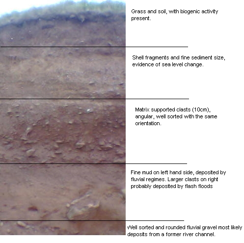
Cliff face
The cliff face shows that the area was previously a lot warmer and humid as there are ferric sediments (Red Fe3+). This warmer period happened just after the last glacial episode, it was caused by Milankovitch cycles, which include:
Obliquity and precession are the two most important factors influencing earth’s climate.
The layers of the profile can be seen in figure 63 where each layer is described.
At lower salinities, there are high levels of nutrients and oxygen. There are also large amounts of suspended sediment here, preventing utilization of these nutrients by the phytoplankton.
Nitrate was found to be conservative throughout the estuary whereas phosphate and silicon exhibit non conservative behaviour. Phosphate experienced addition in the upper estuary due to anthropogenic effects and removal in the lower estuary as a result of biological factors. Silicon on the other hand undergoes net removal due to high numbers of diatoms.
The phytoplankton were found to be dominated by diatoms within the estuary as well as offshore. Chaetoceros sp. were the dominant species in the estuary whereas Rhizosolenia stolterfothii dominated the phytoplankton offshore.
Zooplankton were found to dominated by copepods. The distribution of zooplankton was found to be salinity influenced within the estuary, whereas offshore they were temperature influenced.
The offshore water column was found to be more stratified than that of the estuary. The presence of Eddystone Rocks was seen to have an effect on the mixing processes around this area with turbulent flow occurring on the lee side of the rocks. The estuary itself was found to be partially mixed. The degree of stratification decreased from fresh to saline water. The coastal waters were well mixed.
We have been able to experience and learn from some of the major difficulties involved in collecting data.
Benign dictatorship is a valid method of leadership.
References Back
Blondel, P. and Murton, B.J. (1997) “Handbook of seafloor sonar imagery” Wiley Chichester. pp314
Dyer, K., 1997, Estuaries; a physical introduction. 2nd ed. Wiley and sons. Uk.
Morris, A.W., Bale, A.J. & Howland, R.J.M. 1981. Chemical variability in the Tamar Estuary, South West England. Estuarine, Coastal and Shelf science, 14. 649-661.
Redfield, A.C., 1958, The biological control of chemical factors in the environment: American Scientist, p. 205-221.
Websites
http://www.es.flinders.edu.au/~mattom/ShelfCoast/notes/chapter07.html
http://www.soes.soton.ac.uk/teaching/courses/oa217/(1)courseoutline.htm
Disclaimer: The views on this website do not necessarily reflect the views of the University of Southampton.
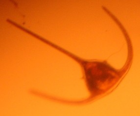 Ceratium tripos
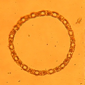 Eucampia
sp
Eucampia
sp