

![]()
![]()
Introducing the Tamar Estuary
![]()
Rock hopping and fault mapping!!
![]()
1 yellow fish, a sea mouse & inshore banking??
![]()
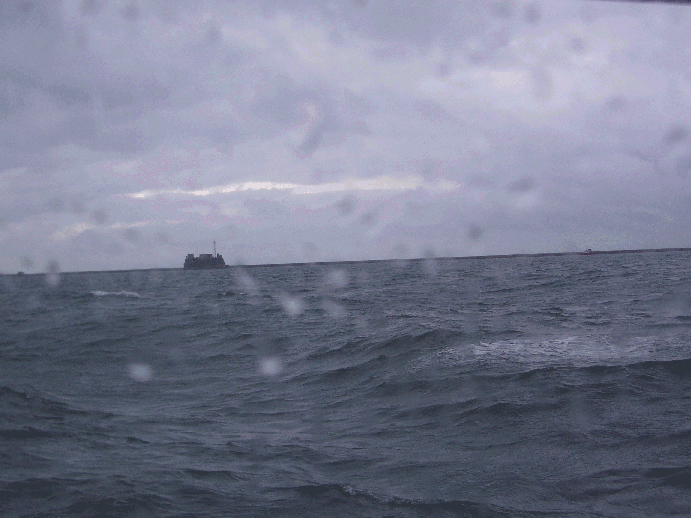
Singing in the rain with the CTD and ADCP
![]()
To Eddystone and beyond ......
![]()
Sun, speed and sampling ........
![]()
Round up of general findings
![]()
|
Figure 1.1 An Aerial photo of Plymouth Sound. |
The area of Plymouth Sound is considered to be a special area of conservation, mainly fed by the Tamar River. The Tavy and the Lynher join the Tamar before flowing into the Hamoaze, out through the narrows and into The Sound. The estuary is generally well mixed due to its shallow nature, however, the water in close proximity to Drake Island fills with hyper-saline water on spring tides due to its 45m depth. The Tamar Estuary is classified as meso-tidal, with a tidal range between 2.2-4.4m on neap tides and 0.8-5.5m on spring tides. Plymouth Sound is protected by a 3km breakwater, which was built in the 19th century. A fleet of ships moored in the harbour were washed onto the rocks as the wind turned southerly overnight. Money came down from parliament to fund the building of the breakwater. On our practical boat days we used a number of vessels and scientific equipment. During the 2 weeks we had four full days out on the water, and a half day investigating the local geology. This webpage is a summation of the results.
|
| Date | Weather | Sampling | Tides |
| 1st July 2005. | Cloudy and rainy. Visibility poor. | Dip/strikes and orientation bearings of
large fold.
Cliff cross section |
07:20 GMT 1.93m
13:40 GMT 4.51m |
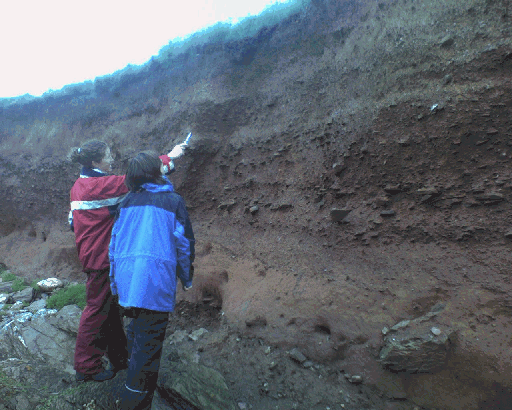
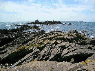 Figure 2.1. The fold exposed at Renny point.
| Introduction The aim was to investigate the processes behind the local geology, and to broaden the view of the estuary from the water itself to the surrounding geological base. The group looked at a large fold/fault system exposed as a wave cut platform at Renny Point. Dips and strikes of the fold were recorded to assess its nature and orientation. A large fault cut the fold and the orientation of this fault was noted to show the direction of its movement. Fractures on the fold were plotted on a compass rose to see how they were related to the fault (this data is displayed in the logbook), allowing us to see if they were dominant or secondary fractures. A large cliff section was also analysed to determine past geological events in the area.
|
Figure 2.2 The recumbent fold at Renny Point |
| Results The fractures along the fold are mainly associated with the dominant fracture. This is shown by the orientation of these fractures on the compass rose. The fractures at 90 degrees to the main fault are secondary fractures. The dips from each side of the antiform showed it to be at an oblique angle. The hinge of the fold was plunging south orientated at 216۫. It was noted as a recumbent fold, due to this angle. The cliff section was a rusty colour and had many distinct layers, figure 2.3. It is thought that after the last glacial maximum 1600 years ago the temperatures began to increase. These temperature fluctuations on large time scales are driven by Milankovitch cycles, (these are patterns in radiation received from the sun related to the Earths proximity, precession and obliquity). Following the melting of ice which covered much of Britain the land was left barren. There was little vegetation, but a very active water cycle. This made the land susceptible to mass movement. The rusty colour, previously mentioned is indicative of a warmer climate at a maximum of 8000 years ago, and the layered cliff is the likely remains of an ancient mudflow. The sediment was of clear horizontal alignment, as a result of shear forces in the flow. Horizontal alignment is the position of least friction. This massive scale mudflow was a combination of high rainfall and lack of vegetation. The sediment was poorly sorted and immature, this excluded the likeliness of much transport, again supporting the mudflow hypothesis. There were also layers of shells at the top of the exposed cliff, suggesting either variations in sea level and/or land rising, or alternatively that they may be deposits from birds feeding on the cliff. Gaining an understanding of the processes which sculptured this section of coastline was an important starting point from which to consider the area surrounding the estuary. Although this was different from the other oceanographic work it is an important reminder that the substrate of estuarine basins can influence the water characteristics.
|
Figure 2.3 Profile of the cliff at Renny Point |
|
|
| Date | Weather | Sampling | Tides |
| 2nd July 2005 | Full cloud cover, rain and very poor visibility. | Van Veen grabs, pipe dredges and Sidescan sonar | 08:20GMT 1.95m 14:40GMT 4.51m |
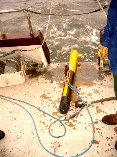
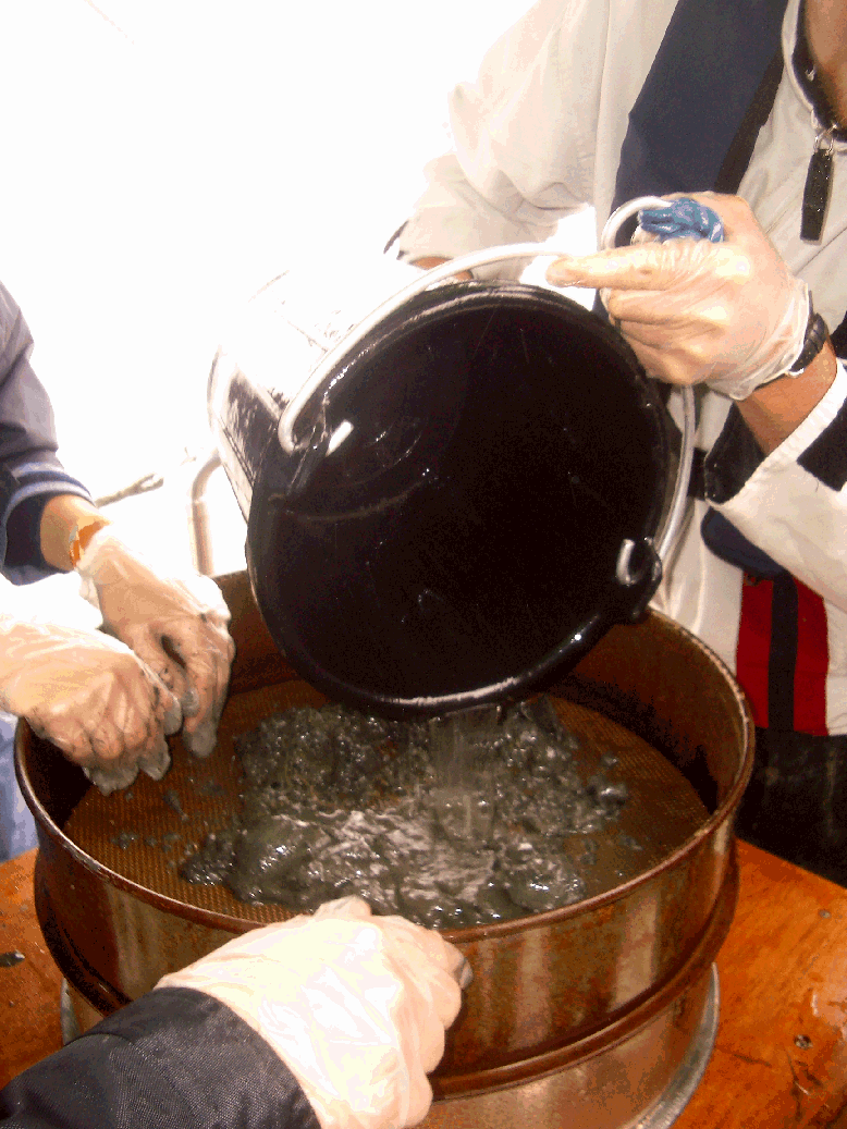
Figure 3.1 The sidescan sonar fish Figure 3.2 A grab sample
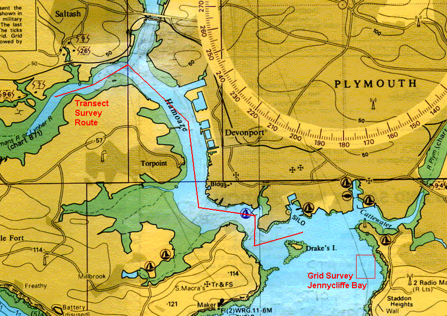
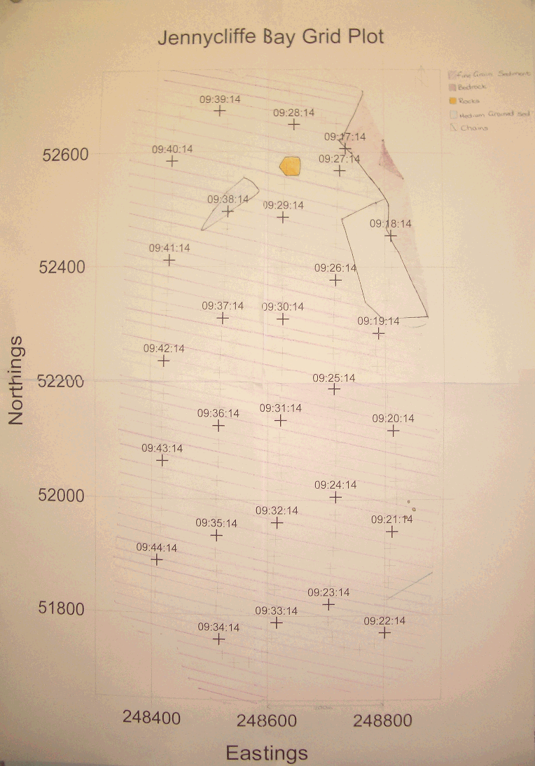
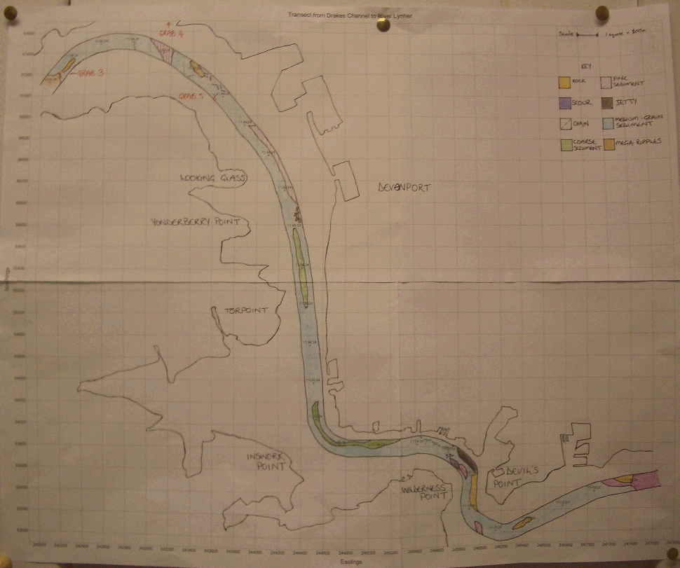
| Introduction The aim of this exercise was to conduct a detailed survey of the bed-forms, bed-types and benthic habitats within the Tamar Estuary and Plymouth Sound. To achieve the above aim, two clear objectives were set. Firstly to complete a grid survey using sidescan sonar of Jennycliffe Bay (050°21.023'N, 004°07.058'W) to (050°20.082'N, 004°07.058'W), in the east Plymouth Sound and to investigate bed types and benthic macrofauna. Secondly to complete a transect survey using sidescan sonar starting from (050°20.082'N, 004°07.058'W) Drakes Channel through The Narrows and Hamoaze sections of the Tamar estuary to the mid-reaches of Lynher estuary (050°23.046'N, 004°13.066'W). Pipe dredges were used to allow examination of the bed types and benthic macrofauna present. The locations of these two surveys are displayed on the chart figure 3.3. The three day predictive weather forecast showed a series of fronts moving in from the Atlantic Ocean over the western British Isles. The wind was set to increase throughout the day, and did, from 7 to at least 15 knots. Calmer conditions in the morning allowed the survey of the more exposed Jennycliffe Bay area with 2 grab samples taken using a Van Veen grab to identify macrobenthic species present and sediment types. The second sidescan transect was conducted in the afternoon through the lower reaches of the River Tamar estuary. The pipe dredge was used to take samples at three locations along the transect in order to compare sediment and biological content, looking for any significant differences between locations.
|
Figure 3.3 A location chart of surveys
Figure 3.4 Weather conditions |
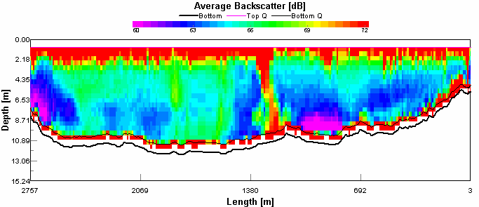
| Results Sidescan sonar The sidescan sonar prints only revealed a small selection of bottom structures. Two plots were made, the first was a grid in the Jennycliffe Bay area, figure 3.5. This had very few distinct changes in substrate. The second was a transect up river, figure 3.6, showing scour holes and some other changes to softer sediment. Flocculation is a major process in the settling of suspended particulate matter input from the estuaries’ rivers, and fine grain deposits can be seen at the convergence of the Lynher and Tamar. There are also fine-grained deposits on the lee of a deep scour hole at the northern end of The Narrows.
One section of the sidescan depicts the large scale bed formations: ‘mega-ripples’, figure 3.7. A mega-ripple is classified as having a wavelength of between 0.6 and 20m (Amos 2003), the bedforms shown were measured to have 3m wavelengths. The mega-ripples formed near to the centre of the channel just seaward of the convergence of the Lyner and Tamar. The structures shown to the right of the mega-ripples are a series of dilapidated metal platforms. It is likely that the restricted flow past the debris covered structures has caused the formation of the mega-ripples. There is little evidence of bifurcation on the image which suggests that there is little wave influence on the bedforms.
Figure 3.8 Scour hole at Devil's Point
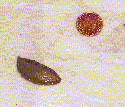
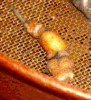
A large anomaly was seen on the sidescan profile at the northern end of the narrows, at Devils Point. figure 3.8. As the sonar scanned the seabed the Natwest II passed over the edge of a large scour hole. Scours are often self-perpetuating and continue to deepen through a positive feedback loop of increased depth leading to increased turbulence and so more erosion further increases the depth. This scour was measured to be approximately 38m deep and has fine grained deposits on its seaward side. The sonar can scan further in deeper water and so the pattern seen is the result of the sonar scanning the other side of the scour hole. The outside bend of the Tamar estuary at Devils Point, where tidal flow energy, wave action and river flow energy are high, shows that the current has eroded down to the bare bedrock, with small deposits of coarse sands sheltered between ridges in the bedrock. Grabs Five bottom samples were taken, two in The Sound with the Van Veen grab and three further up the Lynher with the pipe dredge. The change in the substrate was most noticeable at site 2 in Jennycliffe Bay, where broken slate made up a large part of the sample. Change was also noticeable at site 4 north of the Tamar bridge, where sediment was anoxic, black, lifeless and contained litter. Dredge 3 was taken up the Lynher river and contained only broken shells and Ragworm. Dredge 5 was taken in the vicinity of Bull Point. It contained more life than dredge 3, with more worms, shrimp, bivalves and a common cockle, Cerastoderma Edule. At grab 2 a sea mouse was found, figure 3.9. These live in gravel/shell beds which tied in with the broken pieces of slate also found in this grab. At sites 1 and 2 brittle stars were seen in the grab and grab 1 also contained a starfish a burrowing, siphon feeding bivalve (Arenaria marinata), figure 3.10. These two grabs represented the least anoxic sediment and consequently contained the greatest diversity and quantity of marine life. It is likely that these more oxic conditions are due to better flushing at these sites than further up the estuary . The sewage outfalls are subject to significant dilution by the time the water reaches the open bay. This reduces the pollutants in the sediment and creates better conditions for organisms to survive. Generally it seemed that the best biological habitat was out in The Sound itself. The biology was more diverse here than in any of the samples taken further up the estuary. This may also be due to the more stable temperature and salinity. The salinity in the river is very variable with the tidal flow, however in the Sound itself, conditions are more stable.
|
Figure 3.5 Side scan grid for Jennycliffe Bay
Figure 3.6 Sidescan transect of the River Tamar
Figure 3.9 A sea mouse
Figure 3.10 Arenaria marinata |
|
|
| Date | Weather | Sampling | Tides |
| 5th July 2005. | Heavy rain, with sunny spells at the very end of the day | Phytoplankton and zooplankton sampling, ADCP transects and CTD sampling for nutrients, suspended particulate matter and water flow patterns. | 11:00 GMT 1.65m 17:10 GMT 4.77m |
| Introduction The aim of this day sampling was to investigate the influence of mixing and estuarine flushing on the distribution of nutrients, phytoplankton and zooplankton populations within a dynamic estuarine system. Ten transects were taken throughout the day at key points in the estuary to investigate the processes that are occurring. CTD data was recorded at all of the transects and zooplankton sampling nets were deployed for 2.5 minutes behind the breakwater and north of the Tamar Bridge. ADCP transects were recorded in the following locations:
In addition phytoplankton samples were collected behind the breakwater and north of the Tamar bridge, also in The Narrows at different points in the tidal cycle. This was to investigate how flushing of the estuary affects phytoplankton populations and to investigate any correlations between the biological recordings and the chemical and physical findings. These correlations between the chemistry, physics and biology can then be used to understand the estuary as a dynamic system.
|
Figure 4.1 Weather conditions
|
| Results
The map below (figure 4.2) shows where the ADCP's and CTD drops were taken between the Breakwater and the Tamar Bridge. The map only shows the area covered by RV Bill Conway.
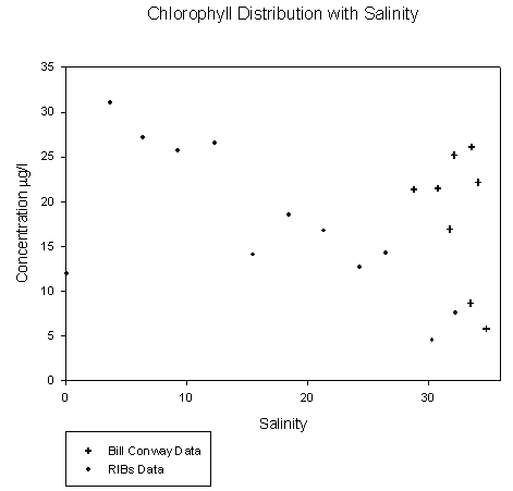
Figure 4.2 Location map of CTD drops and ADCP transects Theoretical Dilution Lines The plot of chlorophyll distribution against salinity see figure 4.4 along the transect of the Tamar estuary did not show the predicted pattern. At low salinities, where fewer phytoplankton were expected, surprisingly high levels of chlorophyll were found, up to 32µg/l . This may be attributed to the use of a fluorometer which cannot accurately differentiate between chlorophyll and suspended sediment when, as is found in the upper Tamar estuary, suspended sediment levels are very high. Interference from these high levels of suspended sediment may have caused the unrealistically high values. Chlorophyll concentration at the higher end of the salinity range, above 29 psu, is elevated to nearly 27µg/l around the site of a sewage outfall (050°24.642'N, 004°12.210'W) which is cleaned of nitrates but inputs high levels of phosphates. At a similar salinity range, in Cattewater, very low chlorophyll concentrations at around 6µg/l are observed This is caused by intense grazing pressure from zooplankton in surface waters detected as backscatter on the ADCP. The theoretical dilution line for phosphate see figure 4.5 over the same transect supports the chlorophyll data, clearly showing elevated phosphate concentrations to 0.0282 µM/l around the sewage outfall at a salinity range of 30-33. Phosphate is generally found in low concentrations in the estuary and so any inputs such as household waste or fertilizers can be significant. Here, phosphate is shown to behave non-conservatively, with some addition occurring near inputs and removal seaward, probably via phytoplankton assimilation. However, even when non-conservative behaviour can be unambiguously deduced, we retain only circumstantial evidence of the processes involved (Morris et.al 1982). The plot for nitrates figure 4.6 on the Tamar transect shows all points remaining close to the theoretical dilution line, indicating generally conservative behaviour. Nitrate is always essentially conserved throughout the upper estuary (Morris et.al 1981). Since the cleaning of nitrate waste from outfalls has been implemented here there has been little addition. Towards the mouth of the estuary and out into Cattewater there is some evidence of the removal due to phytoplankton nutrient assimilation. Silicate figure 4.7 also behaves non-conservatively in the Tamar. There were no significant inputs of silica to the system other than the freshwater tributaries, 30-50% of which are accounted for by the Lynher and Tavy (Morris et. al 1981). Silicate was removed relatively constantly throughout the salinity range. There is one point which lies above the theoretical dilution line, this sample was taken from Cattewater at the mouth of the River Plym (050°21.303'N, 004°09.834'W) and can explained by the rivers fluvial input of silica. ADCP The ADCP data was very extensive and so only a select few samples were examined in detail. These samples were from the following stations: Transect 10 - The narrows (50°21.539'N, 004°10.239'W) Transect 1 - Breakwater (50°20.500'N, 004°10.000'W) Transect 1 The overall velocity magnitude in the water column is shown by figure 4.8, this shows slower flow travelling at < 0.1 metres per second at the bottom due to friction with the sea bed and a faster and more concentrated ebb flow in the western channel of approximately 0.4-0.5 metres per second. The flow is more diffuse in the eastern channel.
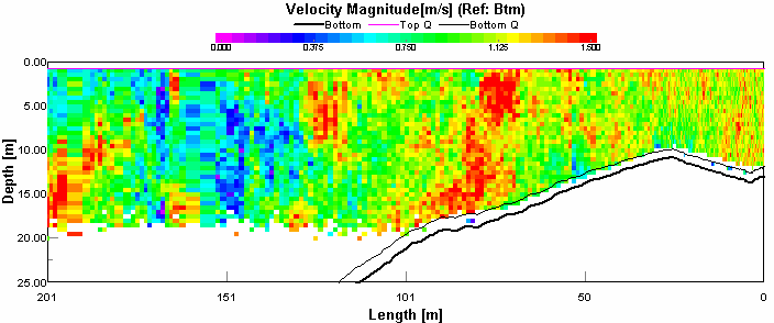
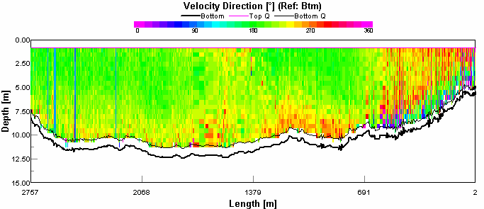
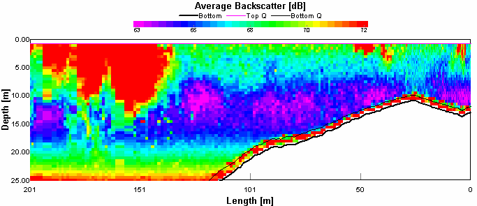
Figure 4.8 ADCP Transect 1 - velocity magnitude Figure 4.9 is showing backscatter, this indicates areas of high turbidity in the water column. It is expected that seawater will have a lower backscatter than river water. This is because river water has much higher concentrations of suspended particulate matter than seawater Seawater is generally colder and more saline than river water, and so will have a greater density and was consequently seen below the more buoyant river outflow. The high surface returns are due to the weather, it was a very windy day resulting in breaking waves introducing bubbles to the water which scatter sound very effectively. There is a column of disturbed water in the middle of the transect which is probably a boats wake. The high return at the sea bed is probably due to the water stirring up sediment. The direction of flow is indicated by figure 4.10. In the western channel the tidal flow is south (180°). This confirms that the transect was taken during an ebb tide. There was a difference in direction of flow at the western shoreline which was travelling south west (270°- 230°). This process also occurred at the sea bed to a varying degree. Most obviously occurring below the ebb tide flow, this is still heading out but was probably being influenced by the bathymetry.
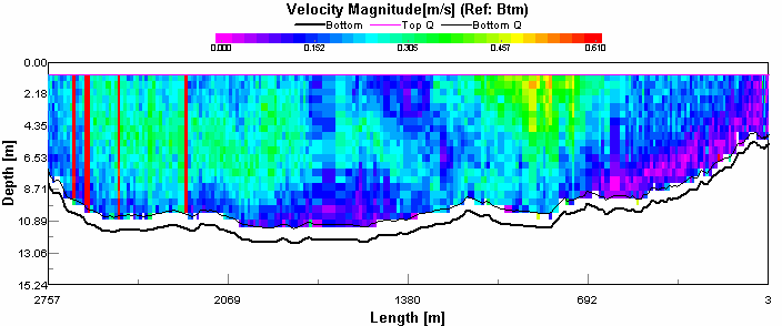
Transect 10 This figure 4.11 shows that there was very high flow here, up to 1.5 metres per second, with flow fastest at the centre of the channel. This will be due to the flood tide through the narrows, as it will speed up through the narrow channel. The area of slower velocity, about 0.375 metres per second was coinciding with a high return on figure 4.12 This may be due to a boats turbulence disrupting the flow. This theory is supported because a ferry passed through the narrows just before the transect started.
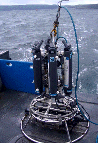
Figure 4.11 ADCP Transect 10 - velocity magnitude Figure 4.12 shows the seawater can also be discerned from the river water as it shows up as lower backscatter, this was apparent between 10 and 20 metres. Above this the river water is creating higher backscatter with its higher sediment load. Below 20 metres there was also a high level of backscatter, this is caused by the fast flow of water entraining sediment from the sea bed. The direction of the flow is very clear; the flooding tide through a narrow channel has caused the water to travel unilaterally, in this case North or 360°. CTD CTD data on the Bill Conway was taken from the Tamar Bridge to the Breakwater using a rosette sampler with 5 Niskin bottles. The aim of the sampling was to understand the structure of the water column under different tidal conditions.
Figure 4.13 and Figure 4.14 Location chart of recorded salinities . The upper chart is a continuation of the lower chart
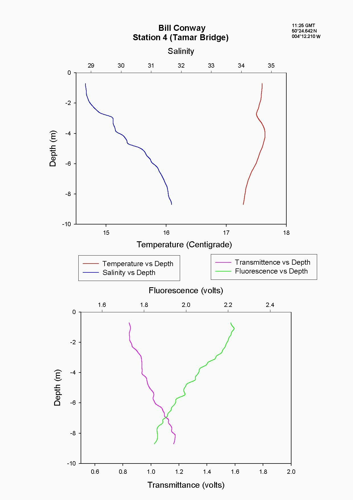
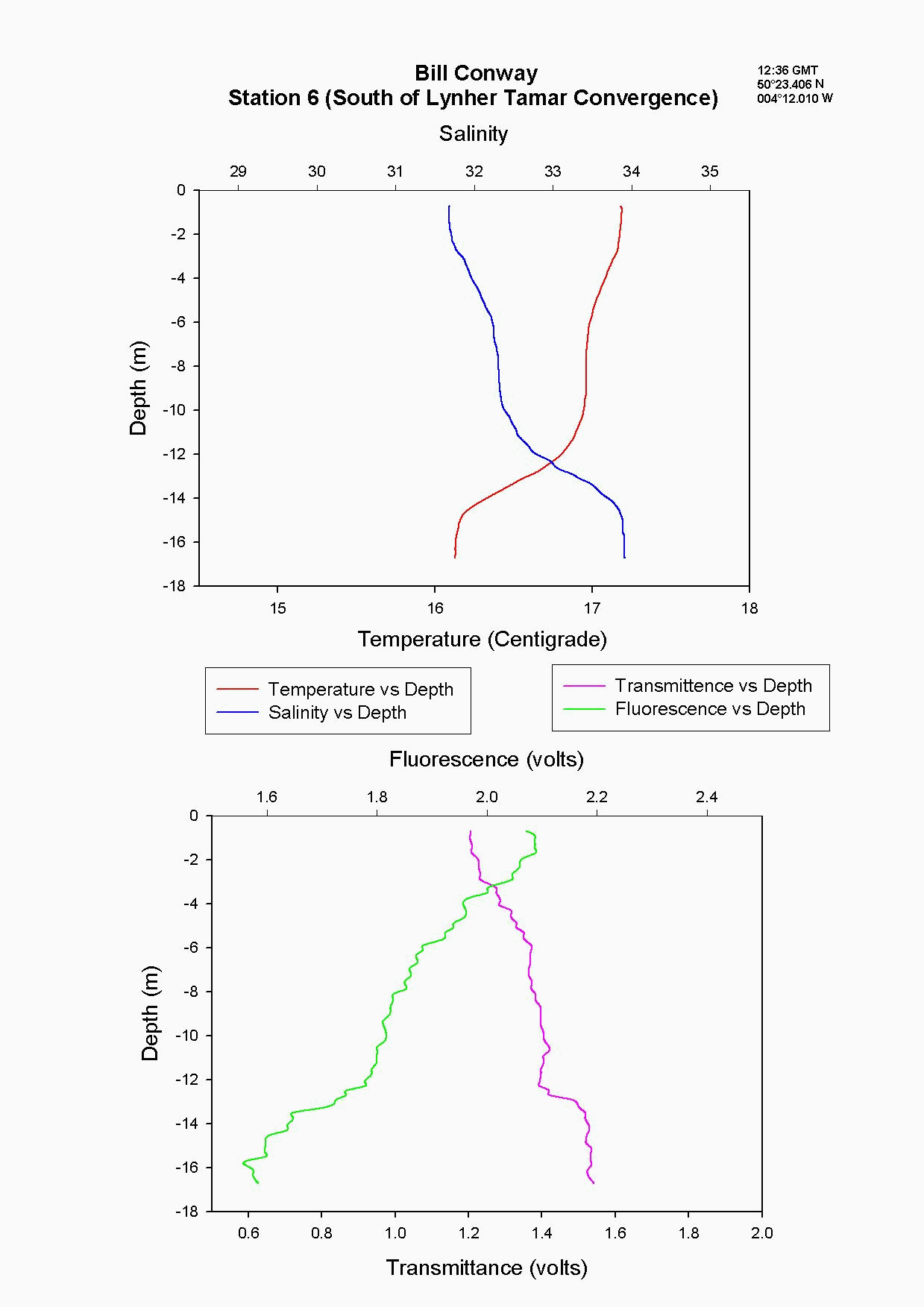
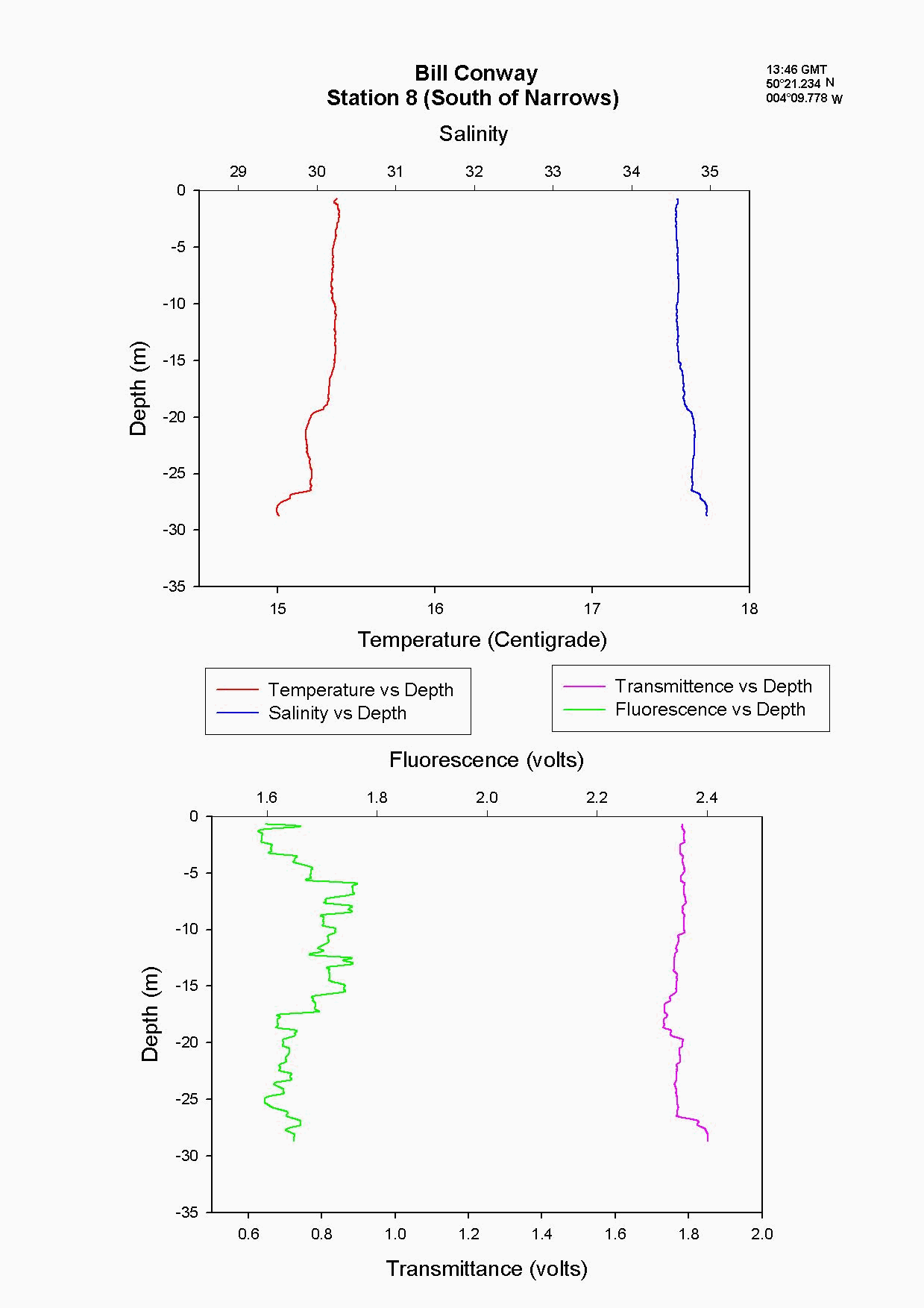
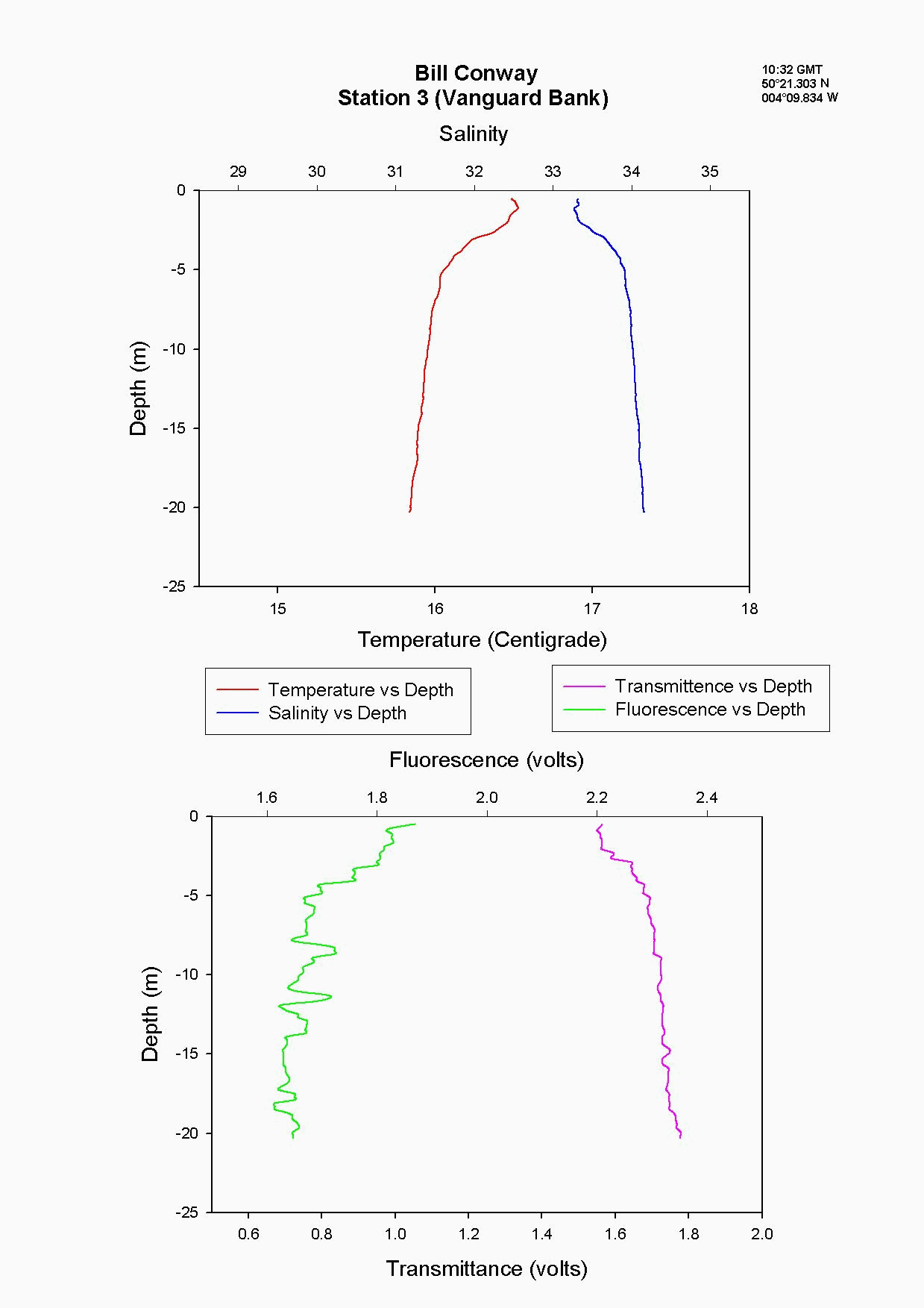
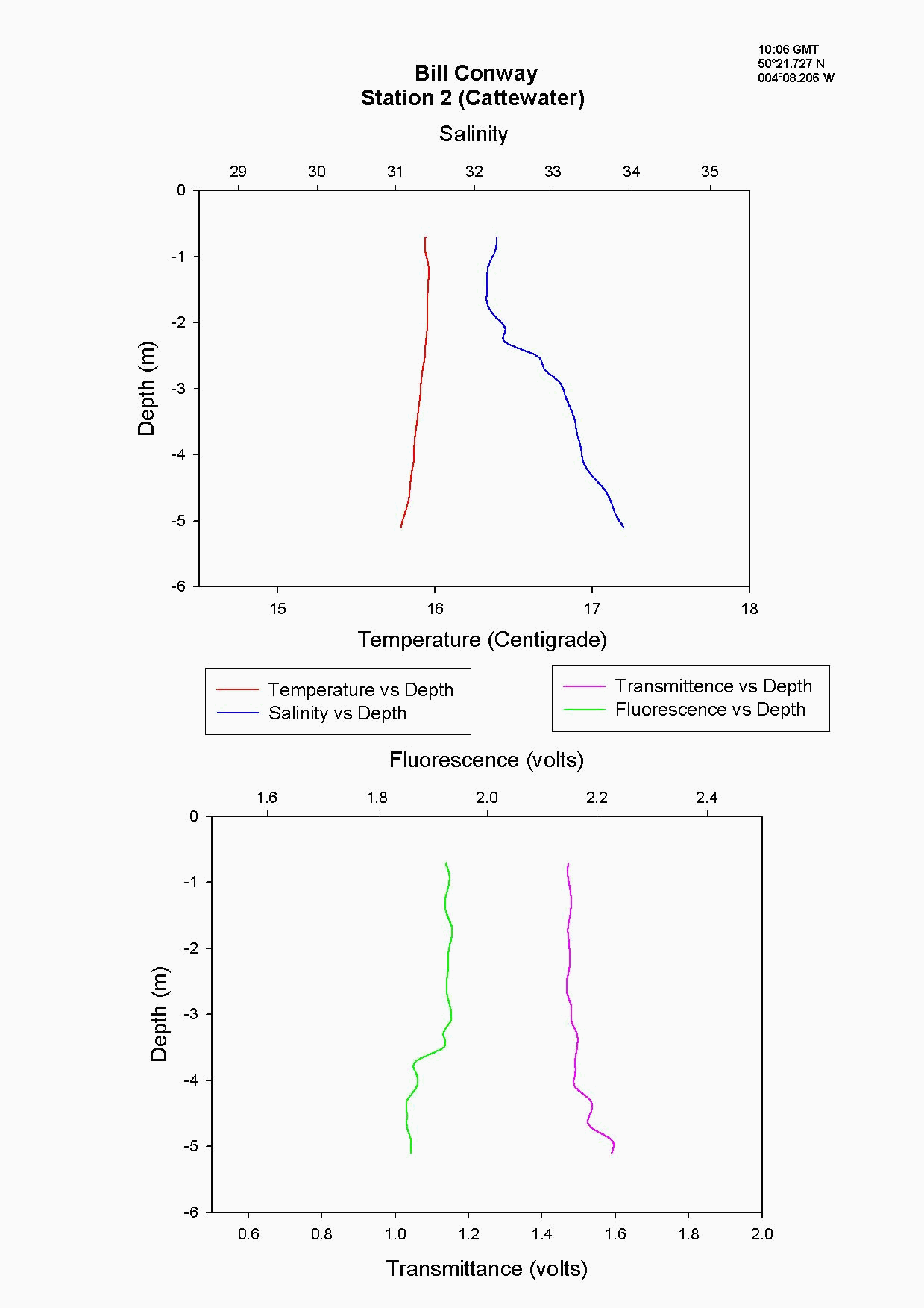
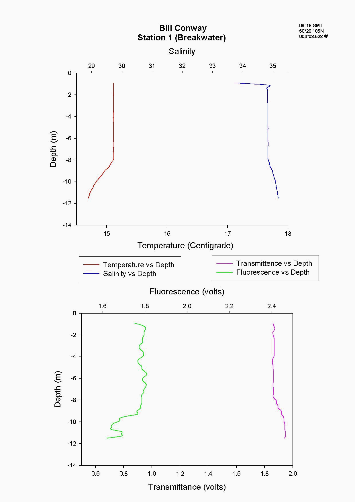
At the Tamar Bridge the temperature decreases with depth and the salinity increases with depth, see figure 4.15 and. At this point the tide was ebbing; the structure seen is due to the lower, more saline layer still pushing up estuary and at the surface a fresher warmer layer beginning to ebb seaward. This gives the sharp change in temperature seen at 3m, it is a change in water body. The higher surface temperature may also be due to a sewage outfall around that area, as the temperature of these outfalls is often higher than the river water. The fluorescence gives an indication of the amount of chlorophyll in the water column, and for this site it was high at 2.2 volts. This should indicate either high numbers of phytoplankton or high sediment, (sediment can interfere with the reading). Phytoplankton data from this site shows it to be 50% lower than most other sites and so it is thought that the high suspended sediment at this site interfered with the fluorescence reading. Transmittance is low here at 1.7 at the surface showing the high particulate matter in the water column. Phosphate levels are also low at this site at 0.026µmol/l, which could be another limiting factor for the phytoplankton. The low levels of zooplankton at the Tamar Bridge are a good reflection of the low numbers of phytoplankton marked by the decrease in fluorescence, and low numbers counted. Further down the estuary (the Lyhner and the convergence of the Lyhner and Tamar) the change in salinity and temperature at a depth of 13m is more clearly defined. This is another profile where the colder salt wedge is pushing up estuary under the warmer fresher surface layer which has started to ebb out, see figure figure 4.16 . The Lyhner and Tamar have medium levels of nitrate, 9µmol/l compared to the Tamar Bridge which had high levels at 19.2µmol/l. However, at the convergence there are high levels of chlorophyll at the surface which then decrease towards the bottom. This is seen in the fluorescence data where below 2m there is a drop in the voltage, this would indicate a drop in the levels of phytoplankton. At the narrows, (station 8) the profile was taken during a flood tide whereas all other stations were sampled during the ebb. The temperature and salinity are constant with depth, this shows stability in the water column down to 20m, see figure figure 4.17 . There is a high amount of noise in the fluorescence data that increases and decreases through the water column to 29m. The transmittance does not decrease in voltage as rapidly compared to the change in voltage of the fluorescence. This is due to the water column being well mixed because of the increase in turbulence. This has been calculated as a Richardson number, and is referred to later. This increase in turbulence is caused by the sudden depth change as the water is confined to a narrower channel. Moving down the estuary from the Narrows to Vanguard Bank the temperature and salinity profiles are seen to change. Salinity decreases and temperature increases in the top 5m but then is constant below that depth as it was in The Narrows, see figure figure 4.18. At Vanguard Bank there is a sewage outfall present. This sewage outfall would give an explanation for the increase in temperature down to 5m depth as sewage outfall is often of a higher temperature. If the water discharge was causing this temperature flux then an increase of plankton would be expected, because phytoplankton feed on the nutrients from the sewage outfalls. Nutrient data shows there is a high level of chlorophyll (26.1 µg/l) and phytoplankton data from this station, (salinity 33.6) shows total numbers to be 175% higher than any other location sampled. It would seem that there is a significant sewage effluent in the surface 5m and this is supporting the massive community of phytoplankton. Below this surface layer the amount of fluorescence decreases, correlating with chlorophyll data showing lower chlorophyll below 5m. At Cattewater, station 2, temperature is constant but salinity increases with depth, see figure figure 4.19. The nutrients in this area are average in the surface layer compared to the others and the phytoplankton data reflects this at a value of 20,000 cells per litre, similar to other sites sampled. The ADCP and plankton data shows high levels of zooplankton at the surface which would indicate that the nitrate at the surface is being taken up by phytoplankton which are then eaten by the zooplankton. At the breakwater, (the furthest point of sampling), there are the beginnings of formation of a thermocline at 8m depth, see figure figure 4.20. The salinity also reflects this thermocline at 8m with an increase of 0.3. Transmittence is high here, at 2.4V, showing good light penetration and as at Cattewater fluorescence values are average. This corresponds with phytoplankton data giving average numbers of 200,000 cells per litre. The average population of plankton on this area may be due to the nitrate which is often depleted in the surface layer and in excess below the thermocline. The fluorescence is lower here at less than 1.8V, (compared to 1.9V at Vanguard Bank), suggesting lower phytoplankton numbers, and the phytoplankton data does show 175% less phytoplankton here than at Vanguard bank. The plankton data shows a change in species at this site and this could be due to an increase in more mobile species which can move below the thermocline to obtain nutrients and then move back up into the surface layers to benefit from the light. There is an increase of Guinardia flaccida at 17000 cells per litre which is only seen at this higher salinity site and this is a slightly more motile species. Zooplankton numbers here are higher than at the Tamar Bridge, at 2000per m³, compared to 240per m³. There are increased numbers of copepods, however the population may be limited, by nutrients being trapped below the thermocline and only average numbers of phytoplankton.
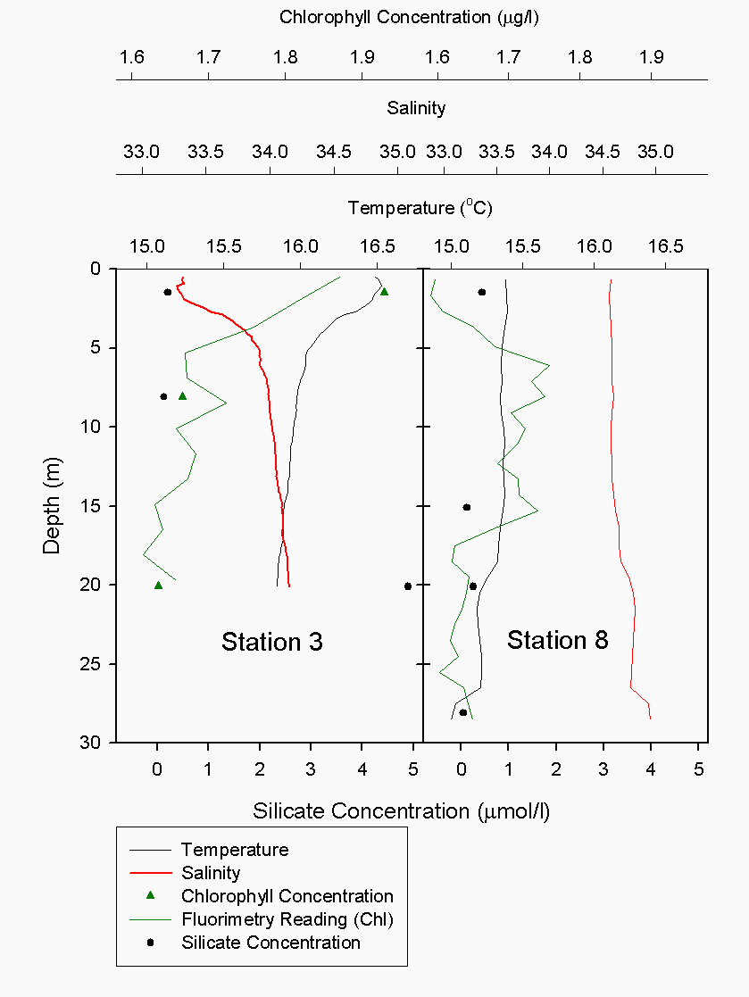
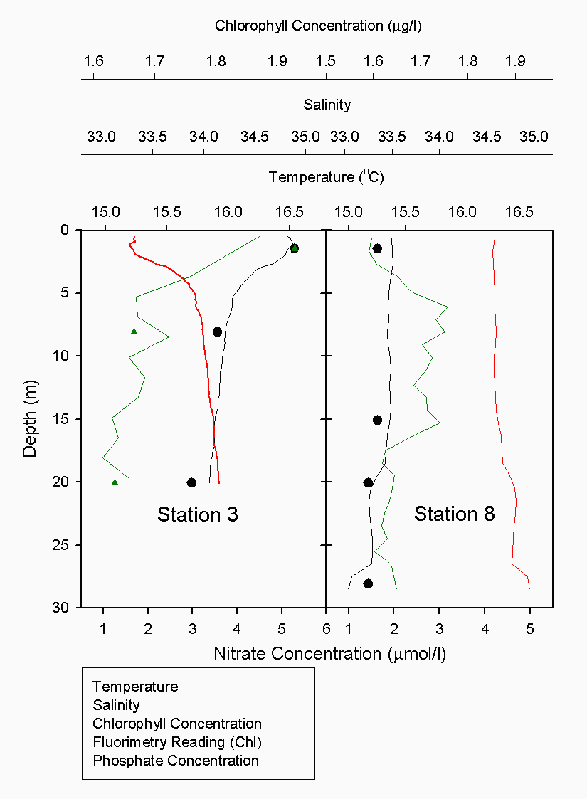
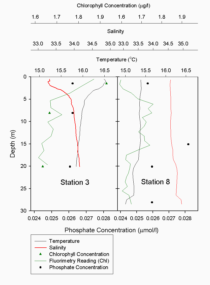
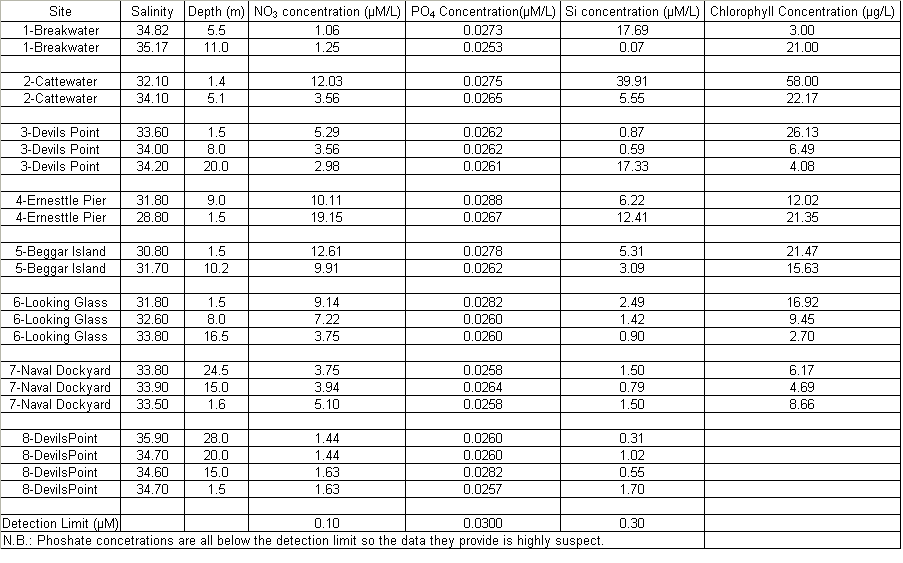
The Richardson number: Stratified water will resist exchange of turbulent momentum between layers due to the density gradient that exists between them. Low levels of turbulence will promote mixing within the layers but will sharpen the density gradient between them because high velocity shear is required for inter-layer mixing. The Richardson number is a measure of stratification versus mixing used to calculate the stability of a water column. The ‘gradient Richardson number’ (Ri) compares the destabilising effects of shear to the stabilising effects of density stratification. The required parameters are gravity, water density (calculated from salinity and temperature), depth and water velocity. These were calculated from the CTD and ADCP data. The Richardson number is defined as: · For Ri > 0, stratification is stable · For Ri = 0, stratification is neutral · For Ri < 0, stratification is unstable and overturning occurs. The Richardson number was calculated for the same two stations sampled at the Narrows, Station 3 was sampled ½ an hour before low tide during a weak ebbing flow, and again (as Station 8), 2 hours after low tide during a stronger flooding flow. The Ri was calculated as: Station 3 = 1.1 Station 8 = 0.1 This shows greater mixing when the tide was flooding, due to a stronger flow at this state of tide breaking down the density gradient. This mixing promotes homogeneity throughout the water column, as shown in Figure 4.21. At Station 8, temperature and salinity are seen to remain relatively constant throughout the depth profile, as does silica concentration. At Station 3 there is some stratification illustrated by a clear thermocline and halocline between 3m and 5m. Silica concentrations are also seen to increase with depth as stratification allows the removal of surface silica by the dominant phytoplankton group, the diatoms. Figure 4.22 plots nitrate against temperature, salinity and chlorophyll. It can be seen from the chlorophyll data that at Station 3 the number of phytoplankton decrease with depth, and therefore it would be expected that nitrate would increase with depth. However, as the tide is in the final stages of its ebb, the surface layer appears to be comprised of relatively fresh water which flows from Saint Johns Lake. This water is ‘muddy’ with high levels of suspended particulate matter giving high surface concentrations of nitrate. At Station 8, when the tide is in flood, nitrate is mixed homogenously throughout the water column. This stratification is less clear for the phosphate data, Figure 4.23, where its distribution throughout the water column is relatively homogenous at both states of tide examined.At the other estuarine stations the nutrient data is summarized in Table 1. For nitrate this showed greater concentrations near the surface than in deeper water (>8m) for all stations. This is illustrated at Station 6 (Looking Glass) where the concentration decreases from 9.14µmol/l at 1.5m to 3.75µmol/l at 16.5m This is likely to be due to freshwater outfalls containing high concentrations of nitrate (such as farmland runoff and sewage outfalls) washing into the fresher surface waters (Pingree et. al., 1984) The continuous addition downstream negates the effects of any mixing occurring. Phosphate appears to remain relatively conservative with depth showing a change of only 0.003µmol/l between the highest and lowest recording. Considering the detection limits for the method used to detect phosphate was 0.03µmol it is inappropriate to analyse these variations in the data. Silicate shows greatest concentrations in shallow waters due to freshwater inputs containing eroded silica from upstream rocks not being mixed to depth. Chlorophyll also remains high in surface waters where irradiance is least depleted and nutrients are greatest due to riverine inputs. Thus providing the best conditions for phytoplankton growth. This does not hold true however for Station 1 (Breakwater) where grazing of phytoplankton by large numbers of zooplankton at the surface and the development of a seasonal thermocline trapping nutrients create a deeper chlorophyll maximum of 21µg/l at 11m depth.
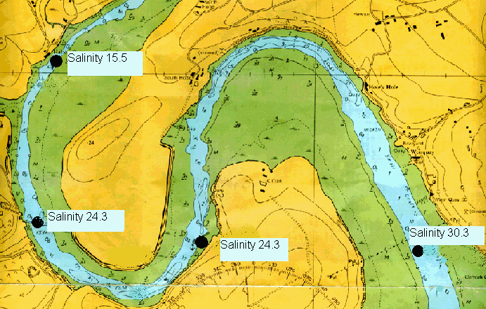
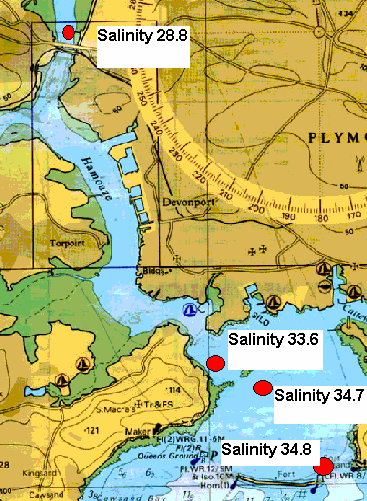
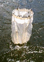
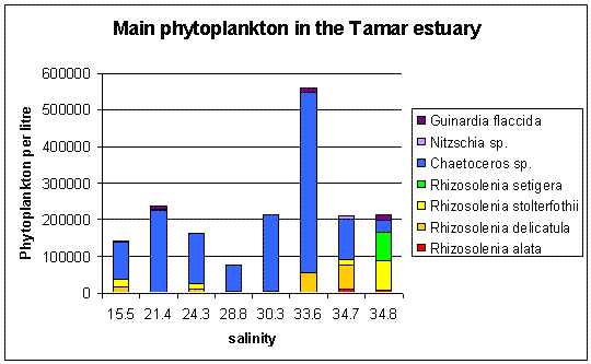
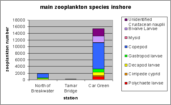
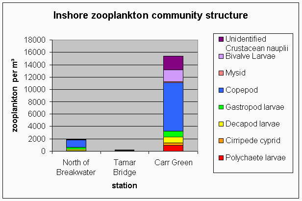
Plankton The plankton data from our trip on the Bill Conway and group 1’s trip on the ribs has been combined to give a picture of the whole Tamar estuary. Phytoplankton samples were taken along the Tamar estuary across a range of salinity values from 15.5 to 34.8 as marked on the map below. Zooplankton samples were taken at one station upstream in the estuary, at the Tamar bridge and the breakwater. Phytoplankton Water samples were taken and filtered and preserved on board using lugols iodine. The samples were then analysed later in the lab. 1ml of sample was analysed each time in a Sedgwick-Rafter tray. The main group found in most samples was Chaetoceros sp., see figure 4.24. The only sample to which this did not apply was the sample taken behind the breakwater, salinity 34.8. The site with the highest total count was salinity 33.6. At the lower salinities the variation in phytoplankton group is much lower. The main group is Chaetoceros sp. There are relatively small numbers of other phytoplankton groups. At salinities 15.5 and 24.3 there are small amounts of Rhizosolenia Stolerfothii and Rhizosolenia Delicatula, however compared to Chaetoceros the numbers are very small at 10-20,000 per litre compared to over 100,000 per litre Chaetoceros sp. The total number of phytoplankton vary for the lower salinities between 150,000 and just over 200,000 per litre. The exception to this was salinity 28.8 where total numbers were much lower at about 80,000 per litre. Salinity 28.8 and salinity 30.3 have the least variance in group, being almost uniquely Chaetoceros sp, 90% and 97% respectively. Salinity 33.6 was at Vanguard Bank near the sewage outfall – this may explain why phytoplankton numbers are around 175% higher here. Growth of phytoplankton requires sufficient supplies of light and nutrients, (Sharples et al, 2001), and nutrients were seen to be higher in this location. This means the water column can support more phytoplankton, as the sewage provides a good nutrient source. Salinity 34.7 was by Carew Point. The main change from the last location to this location was the 175% decrease in total number from Vanguard Bank, and an increase in Rhizosolenia Delicatula. There is also an appearance of Rhizosolenia Alata at 12000 cells per litre, which had not occurred in the estuary until this higher salinity. Salinity 34.8 second was by the breakwater. At this boundary the dominant species changed to Rhizosolenia Setigera and Rhizosolenia Stolterfothii which make up over 2/3 of this sample. Another change at this location was that Rhizosolenia Delicutula, which had been present at most other sites was not present here. The breakwater is in the more exposed bay area and this could be the reason for the changes in species as the water becomes more dominated by the sea and not the sheltered estuarine environment. This can be compared to offshore sampling. The offshore data sample from L4 does show high concentrations of Rhizosolenia Setigera and Rhizosolenia Stolterfothii. Guinardia Flaccida is seen in the offshore surface sample at high concentrations of 6,000 cells per litre out of a sample total of 20000 per litre. Guinardia sp. is also seen here in the sample taken from behind the breakwater at a concentration of 17,000 cells per litre. Zooplankton Zooplankton were collected with a net of mesh size 200µm at the Tamar Bridge, behind the breakwater and at Carr Green, see figure 4.25. The sample was preserved in 10% Formalin so that it could be analysed on returning to the lab. The sample was counted using 2ml samples in a Bogaroff tray and this was repeated 5 times and then scaled up to give an average count per m³. There were much greater numbers of zooplankton from Carr Green compared to the Tamar Bridge and the breakwater, this is shown clearly on the graph where Carr Green has 650% more zooplankton. There were almost 8000 copepods per cubic metre at Carr Green but only 1000 per m³ and 20 per m³ at the Breakwater and Bridge respectively. This difference could be due to patchiness. In assessing copepods in particular, this is very important. They are often found in clusters and one patch of water could be very different to a station only 10 meters away. Carr Green was still at a relatively high salinity of 20, compared to the salinity of 28 measured at the Tamar bridge. Another possible fault is different people counting can lead to errors, or possibly even calculation error. As well as crude number differences between Carr Green and the other two stations, there were also differences in species. There were many Crustacean Nauplii and bivalve larvae in the upstream sample, each at about 2000 cells/litre but there were none or very few at the breakwater and the Tamar bridge.
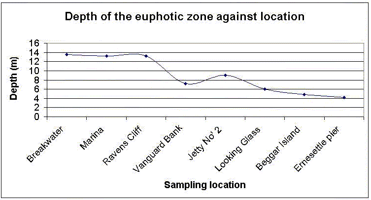
Bill Conway Secchi depths
Figure 4.26 Illustrates the depth of the euphotic zone recorded from the Bill Conway. The sampling stations are in order from the most seaward location at the breakwater up to Ernesettle pier at the riverine end. A Secci disk was used to record the depth of light attenuation this was them used to calculate the depth of the euphotic zone. This figure also shows that the water at the seaward end allowed greater light penetration, the levels gradually decrease in a riverine direction. The increase in light attenuation is due to increasing levels of suspended matter in the water column that gradually settle out through flocculation seaward.
|
Figure 4.3.1 A Phytoplankton net
Figure 4.3.2 CTD Rosette with Niskin bottles
Figure 4.9 ADCP Transect 1 - backscatter
Figure 4.10 ADCP Transect 1 - flow direction
Figure 4.12 ADCP Transect 10 - backscatter
Figure 4.24 Phytoplankton in the Tamar Estuary
Figure 4.25 Inshore zooplankton community composition
Figure 4.26 Depth of euphotic zone
|
|
|
| Date | Weather | Sampling | Tides |
| 9th July 2005 | Glorious sunshine, clear skies and calm sea. | ADCP transects, CTD drops, Niskin rosette, nutrient sampling and zooplankton trawl. | 07:20 GMT 4.97m 13:30 GMT 1.34m |
|
Introduction This practical took place on the 15m research vessel 'Bonito'. The aim was to examine the structure of the water column in a transect from behind the breakwater to the offshore oceanographic station E1, paying particular attention position and effects of the seasonal thermocline. Water samples, a CTD profile and a zooplankton trawl were taken just north of the breakwater (050º20.173'N, 004º09.431'W) before venturing on to station E1, where the measurements were repeated. ADCP profiles were taken throughout the entirety of the day and significant areas examined in more detail. From E1 we headed back stopping at Eddystone Rocks (050º10' 961N, 004º16.698'W) and oceanographic station L4 sampling nutrients and using the CTD at a range of depths. These locations are shown on figure 5.1 Stations L4 and E1 are both sites where oceanographic measurements and samples are taken on a regular basis (L4 is sampled weekly, E1 sampled monthly). L4 (050º16.018'N, 004º14.309'W, water depth ~55m) was first sampled in 1989 and weekly samples have been made ever since. The parameters measured include: · Vertical temperature and salinity profile; · Surface temperature; · Total, and size-fractionated, chlorophyll; · Total, and size-fractionated, particulate CHN; · Phytoplankton species and biomass; · Zooplankton species abundance · Mesozooplankton size-fractionated biomass · Copepod egg production, particularly Calanus helgolandicus · Benthos · Nutrients Regular sampling of E1 (050º05.271'N 04º19.710'W) began in 1902 by the MBA but funding was withdrawn in 1987. Since 1989 when L4 investigation began, E1 has been sampled just once monthly. www.uib.no/jgofs/time-series/LTTS.html www.pml.ac.uk/l4/location.html
|
Figure 5.1 Map to show offshore sampling locations |
| Results
CTD The CTD provided information regarding the structure of the water column at particular sites throughout the estuary and off-shore which were important in determining how changes in the structure of the water column influence the biological and nutrient distribution. The information of particular interest was the salinity and temperature structure, fluorescence and LUP (down-welling light attenuation). A fluorometer was used as a tool to indicate the presence of phytoplankton cells in the water column. Phytoplankton cells contain chlorophyll and when pulsed with blue light from the fluorometer they emit light which can be recorded.
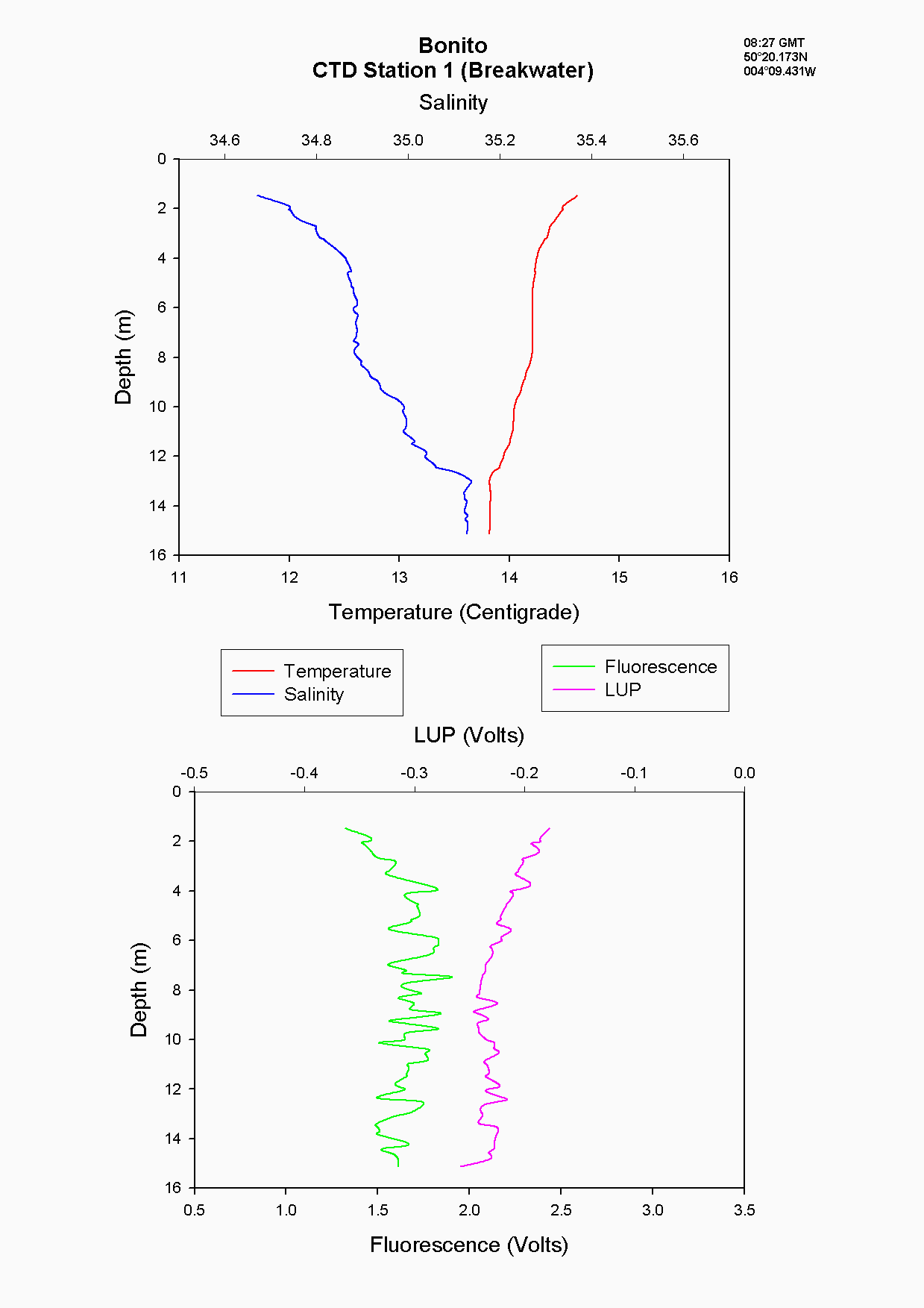
The water column structure inside the breakwater, (station 1), is under the influence of tidal mixing. A two-layer structure was seen with warm, less saline water overlying cold, more saline water which produces a stable water column see figure 5.2. Water column stability within the estuary is determined predominantly by salinity whereas off-shore there is little salinity variation and so temperature determines stability. In addition, the chlorophyll values at the breakwater were very low (0.01 µg/l) when considering the likelihood of nutrients and phytoplankton being trapped and hence building up behind the breakwater see figure 5.3. This may be due to error or possibly patchiness. The boat may have drifted and the fluorometry peak seen when the CTD descended was not actually sampled due to the patchiness.
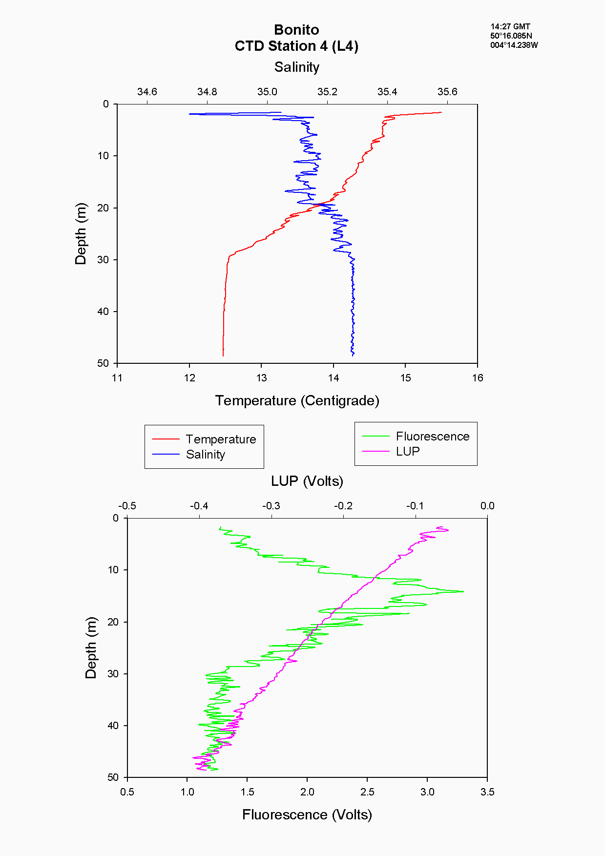
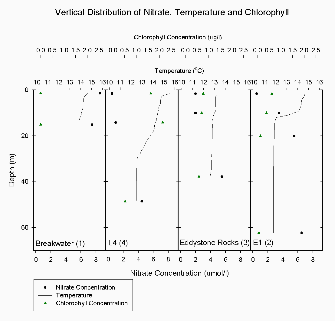
Moving off-shore the salinity values (35-35.2) indicate a more homogenous water column. At the first off-shore station, (L4), there was evidence of a daily thermocline in the upper 2m with the temperature reducing from 15.6۫C to 14.7۫C and a seasonal thermocline which was more gradual than marked, showing a decrease of 2.2۫C see figure 5.4. There is further evidence of a peak in phytoplankton at around 17 m as indicated by the increase in fluorescence on the CTD, an increase in chlorophyll from the discrete samples and an increase in backscatter on the ADCP at the same depth which suggests the presence of zooplankton grazing on the phytoplankton. The nutrient concentrations increase with depth see figures 5.5, 5.6 and 5.7, but as there is a more gradual thermocline than further off-shore, the nutrients were able to be diffused and mixed up into the water column gradually. Essentially, L4 is situated between stratified and transitional mixed-stratified waters (Rodriguez, 2000) and this was evident from the temperature and salinity profiles at this site.
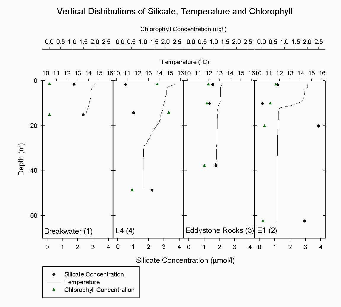
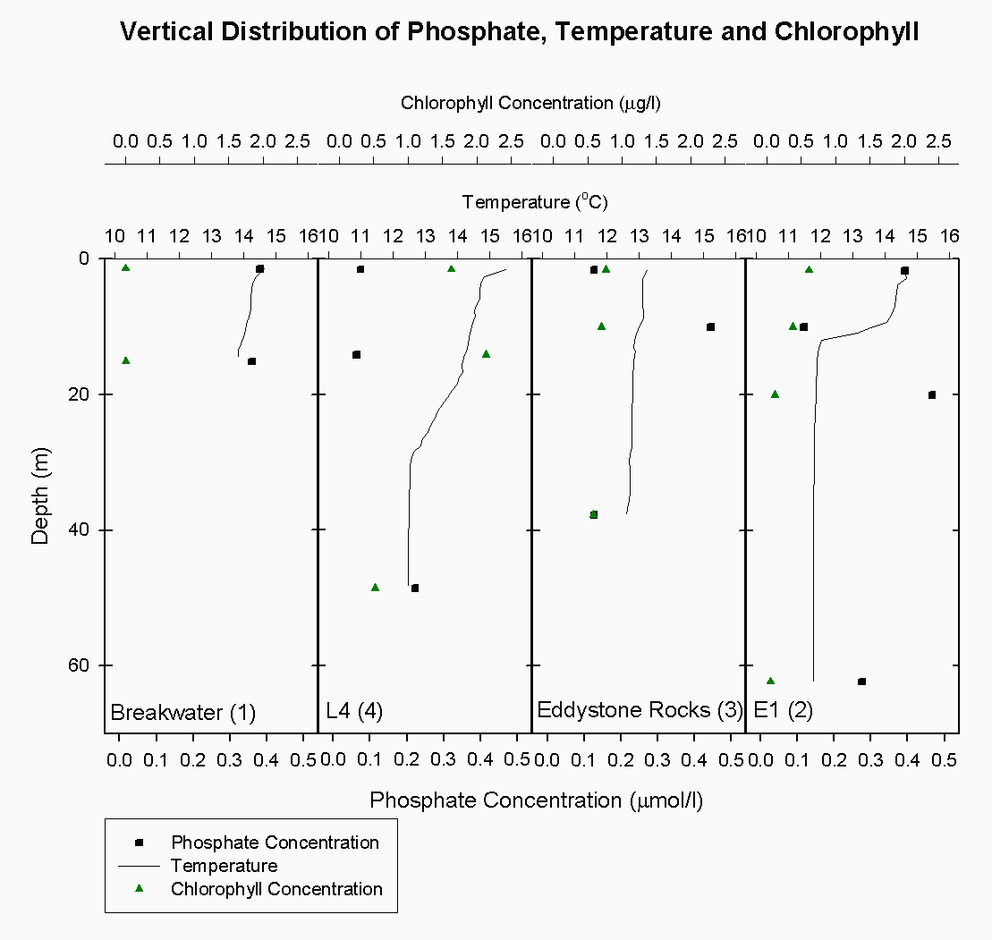
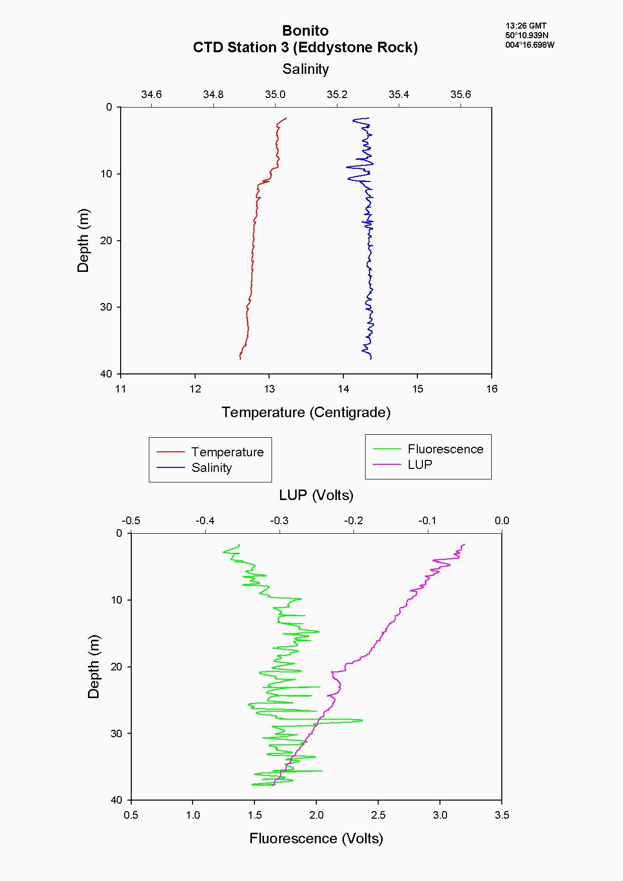
The CTD data at Eddystone Rocks, (station 3), showed a relatively constant temperature and salinity over 40 m depth, although there was still evidence of the seasonal thermocline developing at about 10 m where temperature changes by about 0.3۫C see figure 5.8. This temperature change was not as great as that seen at other stations further from shore due to the CTD drop being taken downstream of Eddystone Rocks on a low slack tide. The water column structure had been broken down over a period of six hours due to turbulence and mixing around the rocks. Silicate concentration generally appeared constant at this depth at 0.9µg/l, whereas nitrate increased from the surface (0.4µg/l) to depth below the thermocline (1.5 µg/l). However, phosphate concentration peaked at 10m 0.5 µg/l to 2.3µg/l which is likely to have been due to a sampling error.
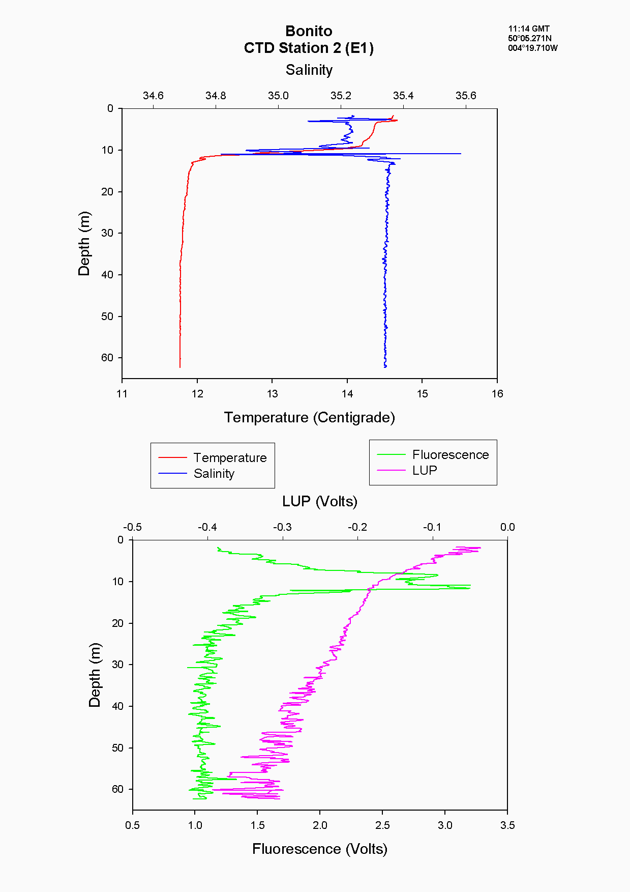
E1 (station 2) was the furthest station sampled from shore at 35.2 km. A marked thermocline had developed here showing a temperature difference of 3 ۫C over about 5m at the seasonal thermocline see figure 5.9. This was due to weak mixing allowing the water column to become more thermally stratified. There was also a marked increase in fluorescence at 10m, where it peaked at 3 volts. This indicates the presence of phytoplankton cells, the dominant species being R. deliculata and R. setigera which are diatoms, also supported by the reduction of silicate concentration at this depth. Diatoms are abundant in this area between April and October (Rodriguez, 2000). Also, the ADCP data again showed an increase in backscatter indicating the presence of zooplankton for the same depth which will utilise the phytoplankton cells figure 5.10. Nitrate continued to increase in concentration, indicating it was depleted in the surface water whereas chlorophyll decreased. The chlorophyll samples are discrete but are unlikely to have been sampled outside this band of zooplankton as this was approximately 10m thick, even considering the off-set in the distance between the sample bottles and fluorometer of approximately 600mm. However, the most likely explanation is that Bonito drifted prior to taking the samples and due to patchiness the chlorophyll peak was not sampled.
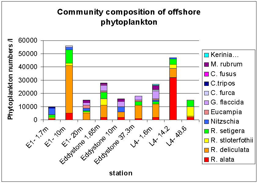
Overall, it is evident that the salinity structure decreases away from the shore and the salinity values increase with distance from the shore. The temperature of the water column decreases with distance from the shore and the water column becomes increasingly thermally stratified. In addition, nutrients become more depleted in the surface water having previously been consumed, but are found in greater concentrations below the seasonal thermocline which inhibits mixing of the nutrients into the upper 10 m of the water column. Subsequently, phytoplankton cells are found at the thermocline where there is still sufficient light for photosynthesis and where nutrients can be consumed from below the thermocline. Offshore sampling of phytoplankton and zooplankton The waters off Plymouth tend to be thermally stratified during the summer months. The degree and extent of stratification is determined largely by water depth and tidal strength. Vertical mixing has a profound influence on the physical and chemical properties of the surface layer which in turn controls the distribution and abundance of planktonic species. At station E1 three zooplankton trawls were undertaken in a vertical profile ranging from 40m – surface. The net used had a 0.5m diameter and 200µm mesh size. The vertical profile showed a change in total species numbers as well as community composition figure 5.11.1The trawl from 40-30m collected the lowest total numbers 338m-3, with Calanoid Copepods dominating the sample. Other significant species at this depth were Hydrozoans, Decapod larvae, Chaetognath and Appendicularians figure 5.11.2 The 15-5m trawl had an increase in total numbers to 357/m-3 and also a change in the relative proportions of the species. Calanoid Copepods decreased in there relative proportion and Hydrozoans and Cyclopoid Copepods increased figure 5.11.2. The 5m- surface trawl collected the greatest number of zooplankton 1033/m-3, double the amount collected in the 15-5m trawl figure 5.11.2. At this depth the population showed greater diversity (see fig 3) with different species appearing prevalent. Appendicularian numbers increased from 19/m-3 in the 15-5m trawl to nearly 383/m-3 in this trawl, and Decapod larvae showed an increase from 6/m-3 at 15-5m depth to 128/m-3 near the surface. Phytoplankton offshore The phytoplankton community was sampled by attaching Niskin bottles to the CTD rosette; this allowed accurate sampling from a number of depths at each location. Three locations were sampled from Bonito; ‘E1’, ‘Eddystone’ and ‘L4’ at these locations three depths were sampled to represent the plankton distribution throughout the water column. Station ‘E1’ is the furthest offshore; samples were taken at depths 1.7m, 10m and 20m. At 1.7m depth 10000/l-1 were counted, the lowest count at this station. At this depth Nitzschia are dominant with R. setigera and R. alata also present. Nitzschia composed 50% of the community. The 10m depth sample shows a large increase in overall numbers to 55,000/l-1. There were also significant increases within individual groups especially, R. deliculata to 36000/l-1 and R. setigera to10000/l-1figure 5.12 At the ‘Eddystone’ station the depths sampled were 37.3m, 10m and 1.65m. The deep sample contained a large proportion of R.deliculata (more than 50% of the total community, 10000/l-1) with R.setigera and G. flaccida also present in high numbers (3000 l-1 each). Overall counts were similar in the 10m sample as the deep sample but with a differing species composition. Here the number of individuals was more evenly distributed between 5 groups R.alata, R. deliculata, Nitzschia, G. faccida, and M. rubium. The surface sample showed an increase in overall numbers to 28000/l-1, with R. deliculta accounting for up to 30% of the community. R. stloterfothii are also present in large numbers with 5000 l-1, which is interesting as they were not found further down the water column figure 5.12 At Station ‘L4’ the first sample was taken from 48.6m, this contained 7000/l-1 R. stloterfothii, 5000/l-1 R. setigera 2000/l-1 R. alata and 1000/l-1 R. deliculata. Overall counts were significantly lower than the other samples from this location; however they are similar to the deep samples collected from E1 and Eddystone. The sample from 14.2m contained 47000/l-1 and was heavily dominated by R. alata containing over 30000/l-1. The rest of the population was made up of R.deliculata, R. stloterfothii and R. setigera. The sample taken from 1.6m contained 27000/l-1. R. deliculata and G. flaccida are the dominant species making up over 55% of the population. Tidal mixing on the continental shelf in the south-western approaches to the English Channel produces a situation in the summer where within a few miles the warmer surface water becomes completely mixed with the underlying colder water (Pugh & Forster, 1975). The frontal region represents an area of recently stabilised mixed water in which a combination of high nutrients and a shallow upper mixed layer create conditions suitable for the rapid growth of phytoplankton (Pugh & Forster, 1975). Temperate waters undergo dramatic seasonality in plankton productivity. The spring diatom bloom is initiated by the initial stabilisation of the water column in deep waters (at E1), or by the increase in light intensity in shallow mixed waters (Kiørboe, 1993). This is associated with a distinct peak in productivity of the mesoplankton, hence the relatively high numbers collected throughout the offshore transect. The spring bloom in temperate waters exhausts all available inorganic nutrients in the euphotic zone; consequently the amount of nutrients retained in the euphotic zone during the spring bloom is important to the developing plankton community which is based mainly on regenerated production. Copepods in particular, but also other mesoplankton are important grazers of the spring diatom bloom. Their phytoplankton consumption during this period has implications for the pelagic productivity beyond the immediate accumulation of zooplankton biomass. The larger the consumption of phytoplankton by zooplankton during the spring bloom the larger the biomass of the pelagic community in the subsequent period. New nutrients that are transported into the euphotic zone by localised or temporary mixing give rise to net phytoplankton blooms (Kiørboe, 1993). Turbulence increases advective transport of nutrients to the surface and hence increases the nutrient uptake rate. Turbulent water motion also influences the light environment experienced by suspended plankton by increasing the light intensity variability. Photosynthetic rate is dependent on light intensity; this explains why the highest quantities of phytoplankton are found in the top 20m of the water column.
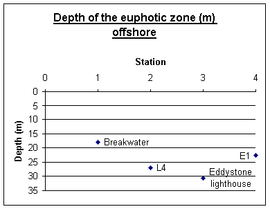
Offshore Secchi disk depths A Secchi disk was used offshore on the Bonito to estimate the depth of the euphotic zone. This was done by the same person each time to avoid judgment error, and is useful as a comparison between sites. The depth of the Secchi disk recorded must be multiplied by three to calculate the depth of the euphotic zone. This is shown in figure 5.13. The Breakwater was the closest station to the shore moving progressively more offshore to E1. The graph shows how the euphotic zone deepens with distance offshore from 18 to over 30 metres. However at E1, the furthest station offshore, light penetration was lower, at 22m. This was due to high numbers of phytoplankton in the water column. At Eddystone Rocks, the deepest Secchi disk depth, phytoplankton was about 20,000 cells per litre, however, at E1 phytoplankton in the surface 10 m was 55,000 cells per litre. This will have blocked out a significant amount of light, reducing the Secchi disk depth, and so reducing the depth of the euphotic zone.
|
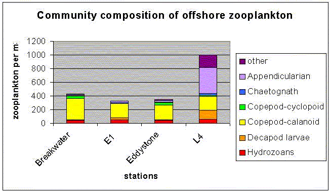 Figure 5.11 Community composition offshore of zooplankton
Figure 5.11.2 offshore zooplankton trawl results
Figure 5.12 community composition of offshore phytoplankton
Figure 5.13 euphotic zone in offshore waters
|
|
|
| Date | Weather | Sampling | Tides |
| 13th July 2005 | Hot and sunny with intermittent cloud | Phytoplankton and Zooplankton, temperature and salinity, nutrients and chlorophyll, oxygen. | 09:50 GMT 3.87m 16:20 GMT 1.00m |
| Introduction The aim of the day on the ribs was to analyse water samples at a lower salinity to complement the data taken on the Bill Conway. Samples and measurements were taken for:
The ribs reached as far up river as Calstock, against an ebbing tide, and the salinity at this point was 3.9. Sampling was then carried out down river at salinity intervals of 4, up to 28, at Carr Green. The zooplankton net was deployed at Carr Green and the light attenuation, nutrients, temperature, salinity and chlorophyll were measured at every station. One oxygen and phytoplankton sample were taken. The weather was dry and sunny and so despite the lack of cover on the working area, contamination should have been minimal.
|
|
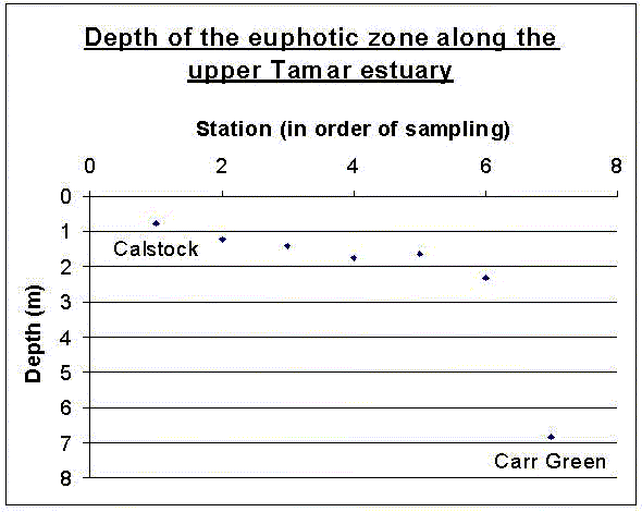
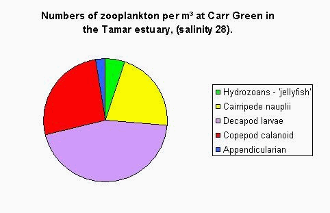
| Results Secchi disk depths Whilst out on the ribs the Secchi disk depth was recorded by the same person at each station along the Tamar estuary from Calstock to Carr Green. It is a simple but useful measurement of light penetration through the water and suspended particulate matter in the water column. The depth of the Secchi disk must be multiplied by three to obtain a depth for the euphotic zone. The euphotic zone depths are shown in order in figure 6.1. The graph shows clearly how the euphotic zone depth increased towards the seaward end of the estuary, the biggest change being from station 6 to Carr Green. In Distance between stations this was the greatest distance, and that is probably why the euphotic zone depth increases so suddenly. The general pattern seen was that the suspended sediment decreased towards the seaward end of the estuary, and so light penetration increased. Where rivers enter the peak of the estuary they are rich in sediment and in the shallow upper reaches this is suspended as particulate matter reducing light penetration. Moving down estuary overall friction decreases as more water is not in contact with the sea bed. This allows settling of sediment and light penetration increases. The expected pattern is reflected well in the Secchi disk measurements takenZooplankton The zooplankton data from the ribs was collected at Carr Green figure 6.2. A 200µm net was used, and as before the sample was preserved using 10% Formalin and then analysed later in the lab. A flow-meter was used to calculate the volume of water passing through the net. The data collected is shown here graphically. There was little variation in the groups found, the main proportion being Decapod larvae and Calanoid Copepods.
|
Figure 6.1 depth of euphotic zone in Tamar Estuary
Figure 6.2 Carr Green zooplankton results |
|
This investigation showed the Tamar to be a partially mixed estuary with a slight salt wedge on a flooding tide, with nutrients often being at higher concentrations in the overlying freshwater inputs and the depth of the photic zone increasing relatively linearly with salinity. With increasing distance offshore thermal stratification becomes more apparent and the effects of the salinity gradient wane. At 30 nautical miles offshore there is a sharp thermocline with nutrient depleted surface waters as a result of the diatom spring bloom. Sediments in The Sound are predominantly muds and fine sands, heavily influenced by the numerous fluvial inputs. Where there was alternative benthic habitat niches appeared exploited and diversity and abundance were high.
|
|
Amos, C. L. 2003. Sedimentary systems and processes. Soes 2013 Lecture material. Grasshoff, K., K. Kremling, and M. Ehrhardt. 1999. Methods of seawater analysis. 3rd ed. Wiley-VCH. Holligan, P. M. and P. J. Williams, D. Purdie, R. P. Harris, 1984 ‘Photosynthesis, respiration and nitrogen supply of plankton populations in stratified, frontal and tidally mixed shelf waters’. Marine Ecology 17:201-213 Johnson K. and Petty R.L.1983 “Determination of nitrate and nitrite in seawater by flow injection analysis”. Limnology and Oceanography 28 1260-1266. Kiorboe, T. 1993. ‘Turbulence, phytoplankton cell size and the structure of pelagic food webs’, Advances in marine biology Vol29 Morris, A. W and A. J. Bale and R. J.M. Howland, 1981. ‘Nutrient distributions in an estuary: Evidence of chemical precipitation of dissolved silicate and phosphate’ Estuarine, Coastal and Shelf Science, 12, 205-216 Morris, A. W and A. J. Bale and R. J.M. Howland, 1982. ‘Chemical Variability in the Tamar Estuary, South west England’. Estuarine, Coastal and Shelf Science, 14, 649-661 Parsons T. R. Maita Y. and Lalli C. 1984 “ A manual of chemical andbiological methods for seawater analysis” 173p Pergamon. Pingree, R. D., and L. Maddock, I. Butler. 1977. ‘The influence of biological activity and physical stability in determining the chemical distributions of inorganic phosphate, silicate and nitrate’, J Mar Biol Ass UK (1977)57:1065-1073 Pingree, R. D. and P. M. Holligan, G. T.Mardell and R. N. Head, 1976. ‘The influence of physical stability on spring, summer and autumn phytoplankton blooms in the Celtic Sea’ Journal Marine Biology Ass UK 56:845-873 Pingree, R. D and P. R. Pugh, P. M. Holligan and G. R. Forster 1975 ‘Summer phytoplankton blooms and red tides along tidal fronts in the approaches the English Channel’, Nature Vol 258 Rodriguez, F. and E. Fernandez, R. Head, D. S Harbour, G Bratbak, M. Heldal, R. P. Harris. 2000 ‘Temporal variability of viruses, bacteria, phytoplankton and zooplanktkon in the western English Channel off Plymouth’. Journal of Marine Biology 80:574-586 Sharples, J, and C. M. Moore, T. P. Rippeth, P. M. Holligan, D. J. Hydes, N. R. Fisher and J. H. Simpson, 2001. ‘Phytoplankton distribution and survival in the thermocline’, Limnology. Oceanography. 46(3): 486-496 http://www.uib.noljgofs/time-series/LTTS.html http://www.pml.ac.uk/L4/location.html
|
 Figure
3.7 Mega-ripples on the sea bed
Figure
3.7 Mega-ripples on the sea bed 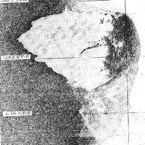


