.gif)
.jpg)

QUICK LINKS
|
-
GEOFIELD |
WELCOME to Group Three's Plymouth Website
.JPG)
Figure 1 - Group 3.
Left to right - Natalie Silverthorn,
Kimberley Bridge, Sarah Karran, Andy Bailey,
Tom Atkinson, Haydn Cooke and Luke Bartrop
QUICK REFERENCE - Click on the boats to view the
practical write-ups
|
RIBs |
BILL CONWAY |
NATWEST II |
BONITO |
Ocean Adventure.jpg) Coastal Research .jpg) |
.jpg) |
.jpg) |
.jpg) |
Introduction
The main aim of the field course was
to study the river Tamar (see Fig.2), it's estuary and convergence with
tributaries and the surrounding coastal area to build an overall view of
the processes dominating each zone and the transition between them. The macrotidal, partially-mixed Tamar is an excellent estuary to study
because a salinity track from 0 to 34 can be made easily by small-boat,
enabling a detailed analysis of the changes involved along the track.
Easy access can also be gained to Plymouth Sound and the surrounding
coastal area, making survey relatively easy for a student field course!
.jpg) |
|
Figure 2 - Map of Tamar estuary |
The field course was undertaken over a 2 week period, with 4 boat
practicals and associated laboratory and data sessions following each
one. The boat practicals and an introductory 'Geofield' practical are
shown in the website below, with corresponding initial findings in the
form of results and analysis. Unfortunately, the resolution of some of
the thumbnails is not exceptional, but by clicking on them and opening a
new window, they should become clearer!
The RIB, Bill Conway and Bonito practicals involved using similar
instrumentation and equipment. A guide to each set of apparatus, as well
as the Sidescan sonar from Natwest II, is shown below. The introduction
to each practical lists which equipment was used in each case.
INSTRUMENT GUIDE
|
SECCHI DISK |
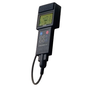
TEMPERATURE – SALINITY PROBE |
|
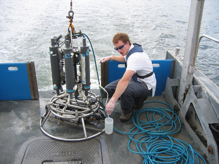
CONDUCTIVITY, TEMPERATURE & DEPTH PROBE (CTD) Measures temperature and conductivity. Water flowing through the conductivity cell is used to calculate salinity. Data is logged via computer. (See figure 6). |
ACOUSTIC DOPPLER CURRENT PROFILER (ADCP)
|
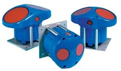
NISKIN BOTTLE 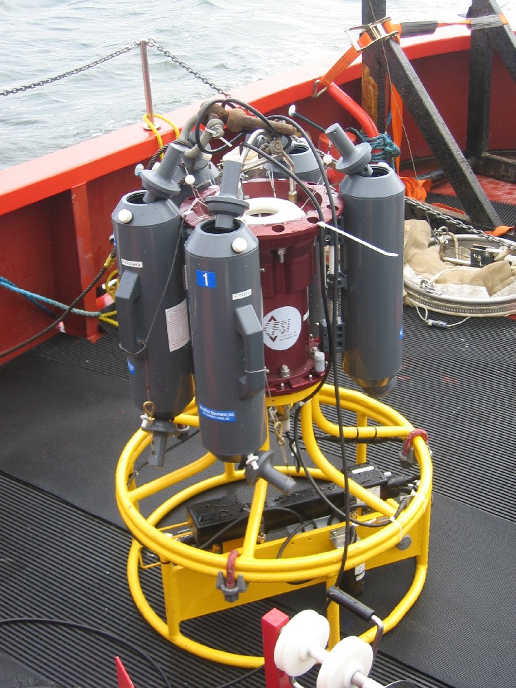 A water bottle triggered by a remote source if mounted on a rosette or a messenger on a line.
Figure 6 - CTD rosette sampler with niskin bottles attatched to the frame. |
PLANKTON NET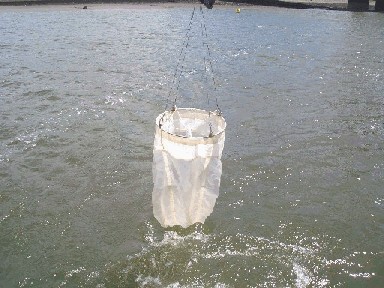 Used
for collecting zooplankton samples. Mesh size used in this case
was 200
µm. The net can either be trawled or simply lowered to a
specified depth for a water column sample Used
for collecting zooplankton samples. Mesh size used in this case
was 200
µm. The net can either be trawled or simply lowered to a
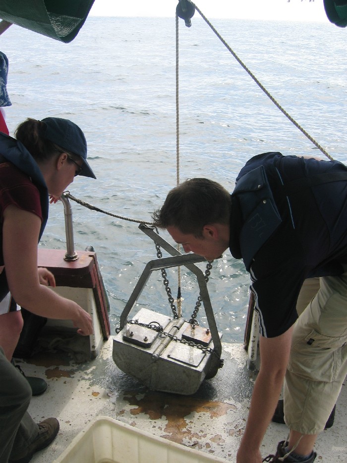
specified depth for a water column sampleFigure 7 - plankton net being deployed |
MINIBAT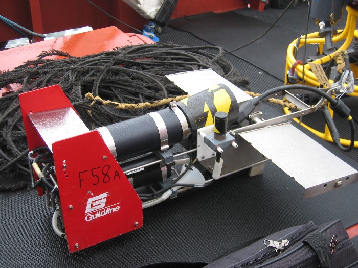 A towed vehicle containing a CTD. It is able to collect a relatively large amount of data over a larger area compared to a CTD mounted on a rosette. Figure 8 - minibat |
|
QUICK LINKS
|
-
GEOFIELD |
Day 1 - 01.07.05 - 1300-1530GMT
GEOFIELD
INTRODUCTION
| WEATHER CONDITIONS | TIDE TIMES | SAMPLING LOCATION |
INSTRUMENTS USED |
|
Overcast (8/8) with scattered showers;
Wind - W F2-3; Air Temperature - 16°; Sea State - Moderate |
DEVONPORT (GMT) HW 1320, 4.5m; LW 0715, 1.7m; 1944, 1.9m |
Renney Point, |
Hand-held Compass and Map of Renney Point |
AIM
The aim of the practical was to study
the bedding, folds and fractures of the rocks at Renney Point as a precursor to the Geophysical survey on
Natwest II.
REPORT
A brief geology
survey was carried out to measure the strike and dip of the rock
structures. The strike is defined as the bearing along the horizontal
line. The true dip is found to be the bearing 90 degrees to the strike.
From the National Geological Survey it can be seen that the main rock
found in this area is Lower Devonian.
The main feature found at Renney Point is an Antiform fold; this is a fold in the rock forming an inverse ‘u-shape’. This particular formation is not perfectly symmetrical and could have been caused due to the rock being pushed up against a more resistant rock. The top of the fold, like many other similar structures, has been eroded away causing overturned bedding to be viewed at the sides of the antiform. Overturned bedding is categorised as rock beds that are past the vertical so they are pointing the opposite way to the other surrounding beds.
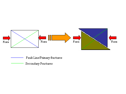
There is a large fault within the rock structure facing out to Renney Rocks with a bearing of 128o. Once looking at the location of the vertical rock strata it can be seen that there has been a shift in the two sides of five metres. This is likely to have been caused by a couple of separate tectonic events, as the force required to move the rock that sort of distance would have to be sizable. The dip of the overall structure is 8o.
Along with the main fault line there are also many dominant fractures which occur around the same bearing as the main fault line (see fig. 9). These occur because the rock is weaker around the fault line so are more likely to break producing dominant fractures. In addition to these are secondary fractures which occur at around 90o to the main fault line.
An analysis of the Cliff face adjacent to Renney Point concluded that there were seven clear separate layers making up the cliff. The seven layers are labelled to the right of figure 10 and annotated in the text below.
 |
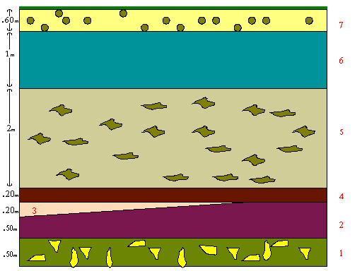 |
| Figure 9 - orientation of primary and secondary faults | Figure 10 - profile of the cliff adjacent to Renney Point |
- Subaerial. Clasts angular ~ 10cm Ø. High velocity flow of post glacial debris due to ice melt in middle Britain 17000 ybp.
- Subaerial. Fine grained mud. Iron rich due to an oxidising environment, such as a delta.
- Subaerial. Matrix supported by laterally discontinuous bed. Small clasts spaced apart ~ 1cm Ø.
- See number 2.
- Subaerial. Larger grained substrate with similarly orientated layered clasts. Laterally extensive. ~ 12,000 ybp earth closest to sun in its elliptical orbit. Described as a stage in the Milankovitch cycle, resulting in melting of glaciers during climate maximum ~8000 ybp. Fast moving mud flows and little vegetation gave rise to the orientation of the clasts.
- Submarine. Sand grains present resulting from possible sea level rise. Tendency of sand to fill river channels.
-
Submarine. Shell fragments visible in sandy
substrate.
BACK TO TOP
QUICK LINKS
|
-
GEOFIELD |
Day 2
- 02.07.05
- 0800-1530GMT
ESTUARINE RIBs
PRACTICAL
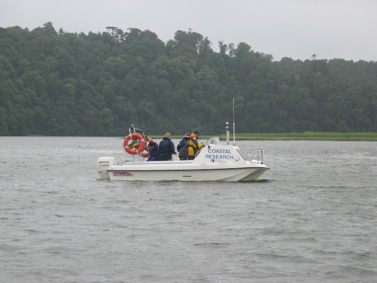
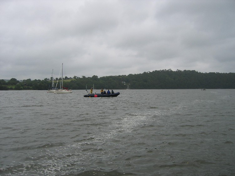
'Ocean Adventure' and 'Coastal Research'
INTRODUCTION
|
WEATHER CONDITIONS |
TIDE TIMES |
SAMPLING LOCATIONS |
INSTRUMENTS |
| Overcast (8/8) - low cloud with scattered fine showers;
Wind - SW F3; Air Temperature - 17° |
DEVONPORT (GMT) HW 0201, 4.5m; 1435, 4.6m; LW 0820, 1.8m; 2049, 1.8m COTEHELE QUAY (GMT) HW 1440, 3.7m; LW 0905, 1.0m |
Calstock |
-
T – S probe - Niskin bottle - Secchi disk - Anemometer - Plankton net (Ocean Adventure only) - Sampling kit (containers, filters, measuring devices etc.) - Boat equipment (GPS/VHF/medical & safety equipment) |
AIM
The aim of the RIBs practical was to
build a profile of the nutrient characteristics of the Tamar, from it's
riverine source (0.2 salinity) down to the 34 salinity water found by
the Tamar bridge. Plankton samples were taken over this area to be able
to explain the nutrient profiles and subsequent estuarine mixing
diagrams.
METHOD
Using calculations from the tidal curve and secondary port data , we estimated the earliest time of arrival at Cotehele Quay (due to the depth of river restricting boat draught) as being approximately 0940GMT. We arrived at Cotehele Quay and, because there was enough river depth and a flooding tide, decided to progress upriver further to Calstock (Station 1). Stations can be seen in figure 11.
The two boats used were 'Ocean Adventure' and 'Coastal
Research'. The group was split into two teams of four and three on the
respective boats. We chose to sample data downstream from Calstock due
to the flooding tide in the estuary and therefore we would be sampling
against the flow of the water ensuring data was not collected from the
same volume of water at different locations on the estuary.
 |
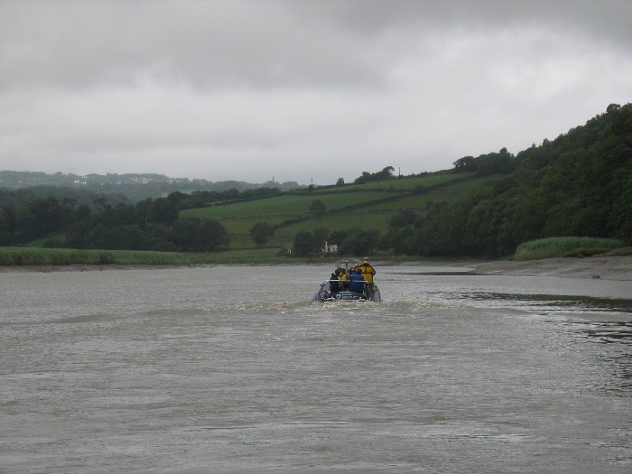 |
| Figure 12 - Natalie, Kim and Tom on the Coastal Research | Figure 13 - Ocean Adventure |
The initial sample was taken at 1130GMT. Data for
salinity, temperature, pH and dissolved O2 percentage were recorded
using the T–S probe. A water sample was taken from each location from
which a filtered volume of 60ml was contained in a plastic bottle (it
was important to use plastic rather than glass in this case to avoid
silica contamination within the samples). The filter was stored in test
tubes with a small amount of acetone to use for later phytoplankton
observation. Transmittance was recorded at various locations using the Secchi disk method.
|
|
|
| Figure 14 - Kev deploying the plankton net | Figure 15 - Salinity front seen at Hole's Hole |
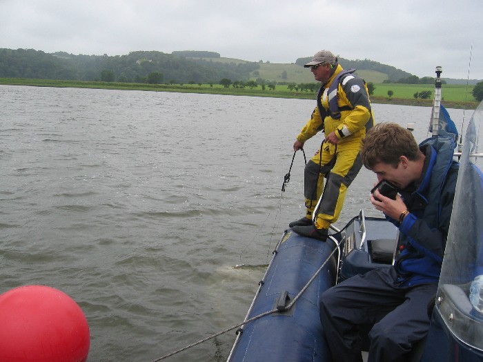
The sampling locations were chosen by salinity rather than geographical location taking a salinity range from, 0 to a value of 32 using an interval of every 2 salinity units. To maximise time efficiency the two RIBs sampled every other location in a leap frog pattern. Oxygen samples were taken at randomised locations to give an unbiased representation of the river profile. These samples were taken by hand using a Niskin bottle. A glass bottle was then filled with the water from the Niskin and allowed to overflow to the same volume to ensure no extra oxygen entered it. The bottle was then sealed and stored submerged in water to avoid contamination. One sample was taken with the Plankton Net (fig. 14). This was done at a mooring buoy on the estuary so as to allow the RIB to turn off it’s engines thus eliminating the possibility of damage to the boat and/or plankton net during sampling. The flow of the estuarine water was great enough on its own to obtain a sample.
The nutrient, oxygen and chlorophyll samples taken were then analysed using the standard techniques which are referenced below:
Manual chlorophyll, dissolved Phosphate and Silicon:
Parsons T. R. Maita Y. and Lalli C. (1984) “ A manual of chemical and biological methods for seawater analysis” 173 p. Pergamon.
Dissolved oxygen:
Grasshoff, K., K. Kremling, and M. Ehrhardt. (1999). Methods of seawater analysis. 3rd ed. Wiley-VCH.
Nitrate by Flow injection analysis:
Johnson K. and Petty R.L.(1983) “Determination of nitrate and nitrite in seawater by flow injection analysis”. Limnology and Oceanography 28 1260-1266.
RESULTS AND ANALYSIS
Plankton
Mesozooplankton: A 420 second tow was taken using the
plankton net, the total population count of the sample was 757393392.
63% of the sample was copepods, 28% Cairripede nauplii and the remaining
9% was made up of Hydrozoans, Bryozoa, Chaetognath, Cirripede cyprid,
Echinoderm Larvae and Gastropod Larvae.
|
|
| Figure 16 - Distribution of phytoplankton along the Tamar |
Phytoplankton: When comparing the phytoplankton
population sizes with data from dissolved PO4 conc. (figure 19) and
dissolved NO3 conc. (figure 18) . A spike in nutrient levels can be seen
at a salinity of approximately 15. A phytoplankton sample was taken at
station 9 which had a salinity of 15.52. This sample consisted
predominantly of diatoms (68%) and dinoflagellates (32%). Station 9 is
situated immediately after a tributary to the river Tamar which could
explain the spike in nutrient levels resulting in a diatom bloom. At
station 14 (sal 24.13) dinoflagellates and diatoms make up
relatively even proportions of the plankton sample with 42% and 58%
respectively. High plankton levels results in a decrease in nutrient
levels especially NO3 conc. PO4 remains relatively high. The pie charts
show that dinoflagellate populations are relatively high at stations 9
and 14 and then drop at the subsequent stations. The chart showing PO4
concentration shows two drops in PO4 concentration after stations 9 and 14 where dinoflagellate populations were high. Diatom populations remain high
throughout suggesting that dinoflagellates use more PO4 than diatoms.
Total populations begin to decrease again after station 15 which as the
Secchi disk results shows is unlikely to be due to a decrease in the
eupotic zone but is most likely to be due to nutrient limitations. From
the samples taken Ciliates were only found at station 15 this could be
because of the salinity range ciliates exist in or more likely it is
because station 15 had the highest population of all the samples and
ciliates were still only counted for a small percentage and therefore it
is possible that they were present in all samples but only showed up at
station 15 due to the higher population size. The high population
numbers at stations 14 and 15 can be seen on the chart for dissolved
oxygen which shows spikes in levels at these locations most likely
caused as a result of increased phytoplankton photosynthesis adding
dissolved oxygen to the water.
Nutrients
ESTUARINE MIXING DIAGRAMS
Estuarine mixing diagrams (EMD)
were produced to determine the behaviour of nitrate, phosphate and
silica down the estuary. Silica, as shown in Figure
17, shows a non-conservative
addition in the upper estuary, salinities 0 to 13, and then a continual
removal in the lower part of the estuary, salinities 14 to 33. The
reasons for this addition and removal cannot be determined directly from
the EMD although explanations may be inferred from the charts and
observations on the field day. Silica sources are typically from the
riverine end member opposed to the seaward end member. The addition of
silica in the upper Tamar estuary may be caused from the large amount of
agricultural land surrounding the estuary, with this in mind it may be
suggested that the high concentrations of silica may be caused by
run-off of agricultural fertilizers and other chemicals that typically
have high silica content. In the lower part of the estuary where there
is continual removal of silica, a number of reasons may be suggested,
including the removal of silica by phytoplankton; more specifically
diatoms that take up high amounts of silica, which is used in test
formation. The concentration of silica in lower parts of the estuary may
be possibly described as being conservative; this then suggests that
silica concentration in higher salinities may also be effected by
dilution in the large amount of marine water.
|
|
| Figure 17 - Silica EMD |
Nitrate concentrations, as shown in Figure
18, show a non-conservative
addition near the riverine end member, at salinities of 0 to 7, in the
rest of the estuary nitrate displays what may be described as a
consistent removal the further you progress down the estuary towards the
seaward end member. Again, reasons for this behaviour cannot be inferred
directly from the EMD although possible causes of the trends could
include the input of agricultural chemicals from surrounding farmland in
the lower salinity areas in the upper estuary. In the rest of the
estuary, in the salinity range of 8 to 33, the consistent removal of
nitrate with the increasing salinity that may be due to the removal of
nitrate by increasing populations of phytoplankton, for instance, at
station 9 with a salinity of 15.5 the plankton sample collected
contained a total population of 1.8x10⁷, whereas further
towards the seaward end member at station 18 with salinity of 32.2 a
total population of 3.6x10⁷. This shows a two-fold increase
in phytoplankton population numbers, which may be associated with the
consistent removal of nitrate as salinity increases towards the seaward
end member.
|
|
| Figure 18 - Nitrate EMD |
Phosphate concentrations, as shown in Figure
19, show a non-conservative
removal towards the riverine end member up to a salinity value of 25 and
then non-conservative addition in the salinity range of 25 to 33. The
reasons for this non-conservative removal and addition cannot be
directly inferred from the EMD although reasons do become clear when the
biology and surrounding land usages are considered, for example, in the
upper estuary, in the salinity range of 0 to 25, phosphate removal could
be due to the uptake of phosphate by phytoplankton species. The
non-conservative addition in the more saline regions, salinity range of
25 to 33 could be due to input of sewage outfall from the sewage
processing plant at Henn Point, which discharges into the Tamar Estuary
south of Coombe Bay. Sewage is discharged on the ebb tide and although
sampling was completed on the flooding tide, the phosphate
concentrations are elevated enough to suggest that some of the phosphate
remained in the estuary after the turning of the tide so creating an
appearance of non-conservative addition in this region.
|
|
| Figure 19 - Phosphate EMD |
DATA
A full set of data can be found at Group3/Ribs020705
BACK TO TOP
QUICK LINKS
|
-
GEOFIELD |
Day 5
-
05.07.05 - 0800-1630GMT
'BONITO' OFFSHORE PRACTICAL
INTRODUCTION
| WEATHER CONDITIONS | TIDE TIMES | SAMPLING LOCATIONS |
INSTRUMENTS USED |
|
Overcast (8/8) with scattered showers;
|
DEVONPORT (GMT) |
Plymouth Sound Figure 21 - Chart of the narrows to the Tamar Bridge with locations of sampling sites |
- miniBAT |
.jpg)
.jpg)
AIM
The aim of the offshore fieldwork was to address the following
question:
‘How do
vertical mixing processes in the waters off Plymouth affect, directly
and indirectly, the structure and functional properties of plankton
communities?’
METHOD
The original plan for the day was to sample an initial station
behind the breakwater in Plymouth Sound
(50˚ 20.129’N 004˚ 09.290’W) for a time series collected at
the same site by all 12 groups. We were then going to head East and
collect samples at set stations in Bigbury Bay, at the mouths of the
rivers Yealm and Elbe. While on route to the Bigbury Bay stations, we were going to tow 'MiniBAT', a device which
collects CTD, Fluorometer and Transmissometer data whilst on the move,
allowing for a large area of CTD data collection in a relatively short
time. Unfortunately on the day, the sea state proved too rough (with large swells) which meant all sampling had to be done within the confines
of the breakwater and up the river Tamar as far north as the Tamar
Bridge (50º 24 480N 004º 12 270W). Trying to deploy the CTD
rosette and miniBAT in the swells outside the breakwater would have
proved too dangerous. Sample sites that were used can be seen in figures
20 and 21.
 |
 |
|
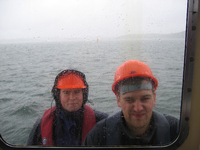
Figure 22 - Haydn and Tom outside in the rain on Bonito |
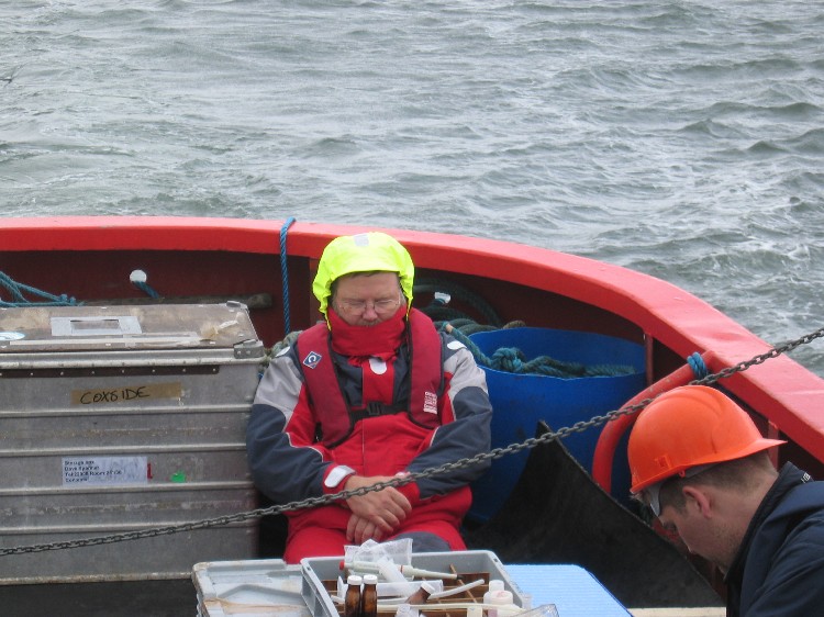
Figure 23 - Been burning the candle at both ends Anthony? |
Below are the
references for the lab procedures which were undertaken to analyse the
samples collected:
Manual chlorophyll, dissolved Phosphate and Silicon:
Parsons T. R. Maita Y. and Lalli C. (1984) “ A manual of chemical and
biological methods for seawater analysis” 173 p. Pergamon.
Dissolved oxygen:
Grasshoff, K., K. Kremling, and M. Ehrhardt. (1999). Methods of seawater analysis. 3rd ed. Wiley-VCH.
Nitrate by Flow injection analysis:
Johnson K. and Petty
R.L.(1983) “Determination of nitrate and nitrite in seawater by flow
injection analysis”. Limnology and Oceanography 28 1260-1266.
RESULTS AND
ANALYSIS
Plankton
In offshore systems the abundance of zoo and phytoplankton is largely
controlled by the vertical structure of the water. Surface waters tend
to be well lit and nutrient poor, while the darker, deeper waters are
nutrient rich. As well as this there may well be temperature
stratification in the form of seasonal thermoclines. As was described
above the adverse weather conditions prevented any offshore sampling on
the day, so the sampling was taken from the breakwater in Plymouth Sound
up to the
Tamar
Bridge. This radically altered the kind of data which was collected
as estuarine systems are controlled by tides and salinity gradients, so
these factors also must be considered when describing zoo and
phytoplankton distribution. Also the limiting factors related to
nutrients offshore do not apply, the River Tamar and its tributaries
provide an excess of nutrients from agriculture, industrial and domestic
sources. In the previous few weeks before the survey was undertaken
there were high levels of precipitation, this would too add to the
available nutrients in the system.
 |
 |
| Figure 24 - phytoplankton diversity for all stations | Figure 25 - zooplankton abundance for all stations |
The first
station was taken north of the breakwater (see map), from the histogram
of phytoplankton abundance (Fig.24) it can be seen that the diatom
population remains relatively stable as you go down the water column.
The number of ciliates seems to increase as depth increases; this
suggests that they may prefer deeper water. The nutrient data also backs
up these findings (Figs. 31 to 35) the levels of NOз are at a low level (for the
estuary); this suggests that the dinoflagellates and ciliates are
removing it from the system. The zooplankton abundance charts (Fig.26)
display a change in species composition from the surface down to 10m;
this could be related to the presence of both a thermocline and
halocline, which form physical barriers that block vertical migration.
The total individual counts of both phytoplankton and zooplankton (Figs.24+25)
show a correlation, when zooplankton numbers are low the phytoplankton
have a higher abundance, this is due to the predator/prey relationship
between the two groups.
 |
 |
| Figure 26 - zooplankton diversity for station 1a | Figure 27 - zooplankton diversity for station 2 |
Station 2
was sampled at Barn Pool (see fig 21), the diatoms there show a high
dominance in the population (Fig. 27) at around 60%, this can also be seen
in the silica levels (Fig. 32), which are low due to the diatom uptake. A thermocline at around 10m (Fig.
39) may be blocking the downward migration
of ciliates, which show a rise in population down to the themocline, but
are far less abundant at higher depths. The zooplankton counts are
dominated by Cirripede’s, who seem to prefer the less saline
conditions from the abundance charts (Fig. 27). There is also a high
number of zooplankton residing at this station, with the phytoplankton
showing a lower abundance (Fig. 25).
 |
 |
| Figure 28 - zooplankton diversity for station 3 | Figure 29 - zooplankton diversity for station 4 |
Station 3
at the mouth to
Saint Johns
Lake displays a thermo and halocline at 4m, high surface
levels of silica (Fig. 33) can account for the lower dominance of diatoms.
But below the clines the silica levels are lower and the diatoms have
greater dominance. Nutrient output from the lake (Fig. 33) provides the
needed food source for the dinoflagellates and ciliates to become more
abundant. The zooplankton count taken at 4m-surface was dominated by
Cirripede’s and Copepods (Fig. 28), but the population is much smaller
than at station 2 (Fig. 27), so therefore the numbers of phytoplankton
cells is higher.
 |
| Figure 30 - zooplankton diversity for station 5 |
Station 4, just south of the Tamar Bridge displayed lower levels of nutrients (Fig.34); this is due to the high numbers of phytoplankton at this site (Fig. 29). The diatom species display around a 90% dominance in the population (Fig. 29), which accounts for the low levels of silica. These high phytoplankton numbers have a dramatic effect on the number of zooplankton present (Fig. 25), which is very low compared to samples further seaward. The diversity of the zooplankton all seems to be related to the salinity as there were only 2 species found at this station with Cirripede’s accounting for the vast majority of the population (Fig. 29).
Station 5
was sampled at the Mayflower Marina and high concentration of nutrients were found, (Fig.35)
especially silica which would explain the lower dominance of diatoms and
the increased numbers of dinoflagellates and ciliates (Fig.30). Again
there is a relationship between the numbers of phytoplankton and
zooplankton, with zooplankton numbers being higher the phytoplankton
show a decline. The zooplankton population at this site shows
a higher diversity than at other sites sampled, this could be due to the
sheltered conditions at the site and the water column is well-mixed
(Fig. 35) from 1m down. There is a surface thermocline, which is due to
the calm wave conditions and sunny weather on the sample day.
Nutrients
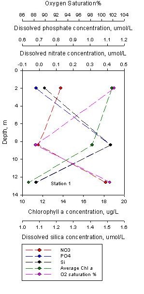 |
STATION 1
The diatom
population remains relatively stable through the water column at this
site. However, as photosynthesis cannot occur below the critical depth,
there is a continual decrease in chlorophyll a concentration
(from ~18.8 to ~10.3 µg/L) – shown at every station. An increase in
Dissolved Oxygen is seen between 8m and 13m (~88 to ~101%). It is most
likely that this increase is seen because there is a peak in
phytoplankton at this depth. The increase in phytoplankton numbers gives
rise to an increase in photosynthetic production of which oxygen is a
product. Nitrate concentrations increase beyond 8m depth after the
chlorophyll maximum.
An
initial increase is seen in both the silica (~1.13 to ~1.52 µmol/L) and
phosphate(~0.68 to ~1.12 µmol/L) concentrations from 0-8m after which a
decrease is seen (silica ~1.52 to ~1.09 µmol/L, phosphate ~1.12 to ~0.67
µmol/L). |
| Figure 31 - Vertical profile of nutrients, dissolved oxygen saturation % and chlorophyll a for station 1 |
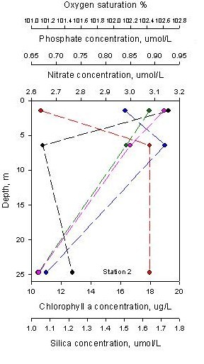 |
STATION 2 We might assume that the upper layer is representative of the euphotic zone and that a decrease in both average chlorophyll a concentration (~17.8 to ~10.2µg/L ) and % dissolved oxygen saturation (~102.6 to ~101.05%) is a result of decreasing light levels below the surface hence less phytoplankton. As the abundance of phytoplankton decreases, so does the level of nutrient uptake explaining an increase in levels of nitrate (~2.63 to ~3.08 µmol/L) and phosphate (~0.84 to ~0.658 µmol/L). The continued decrease in silica (~1.75 to 1.23µmol/L) concentration may be due to uptake by siliceous diatoms as necessary for growth and not photosynthesis. The lower layer contains fewer synthesising phytoplankton and thus less oxygen is produced. |
| Figure 32 - Vertical profile of nutrients, dissolved oxygen saturation % and chlorophyll a for station 2 |
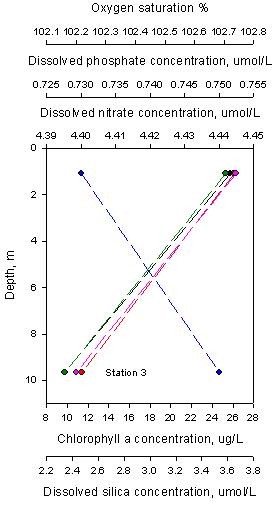 |
STATION 3 Dissolved silica and nitrate concentration decreases ( Silica~3.68 to ~2.30 µmol/L, nitrate ~4.445 to ~4.400 µmol/L) down through the water column. This nutrient uptake is usually representative of phytoplankton, although a decrease is also seen in chlorophyll a concentration (~25 to ~9.9 µg/L) and dissolved oxygen % (~102.75 to ~102.2%). Dissolved phosphate concentration increases (~0.730 to ~0.750 µmol/L ) this could be due to the sewage out fall at Henn Point, which discharges into the Tamar Estuary south of Coombe Bay (North of station 3) or farm land run off. |
| Figure 33 - Vertical profile of nutrients, dissolved oxygen saturation % and chlorophyll a for station 3 |
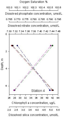 |
STATION 4 A decrease in chlorophyll a is seen (~5.0 to ~2.4 µg/L). This explains the increases seen in all the nutrients with depth, (nitrate ~7.33 to ~7.44 µmol/L, phosphate ~0.770 to ~0.790 µmol/L, silica ~2.03 to ~5.1 µmol/L). As expected due to a reduction in photosynthesis a decrease in dissolved oxygen saturation was observed (~102.5 to ~102.05%). These lower values of phytoplankton could be due to turbulence and disturbance near the bridge from all the traffic that passes under it. |
| Figure 34 - Vertical profile of nutrients, dissolved oxygen saturation % and chlorophyll a for station 4 |
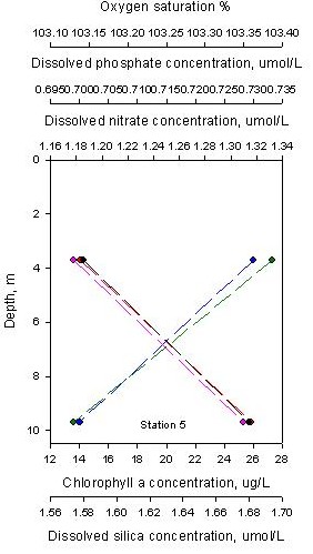 |
STATION 5 An increase in dissolved oxygen saturation % is seen (~103.105 to ~103.350), but unlike at station 1 it is not accompanied by an increase in chlorophyll a concentration (~27 to ~13.8 µg/L). There is an increase in nitrate (~1.18 to ~1.30 µmol/L) and silica (~1.58 to ~26 µmol/L) concentrations with depth, this is easily explained by the decrease in chlorophyll a concentration. Phosphate decreases with depth from ~0.730 to ~0.700 µmol/L. The decrease in phytoplankton with depth could be due to a thermocline or pollution from the marina. |
| Figure 35 - Vertical profile of nutrients, dissolved oxygen saturation % and chlorophyll a for station 5 |
ADCP Profiles
Figures 36 and 37 show a section of ADCP transect taken from an area mid-channel in the East of Barnpool. A strong eddy is found to be present in this area, with an intense area of maximum velocity of 0.5ms-1 moving southwards in the deeper part of the water column at a depth of 17m to 30m, with a reduced velocity of 0 ms-1 to 0.125ms-1 moving northwest to north nearer the surface at a depth of 0m to 17m. This transect was taken from south to north, so the higher intensity area may be said to be further south than the area of lower intensity. This is due to the ebbing tide forcing water out of the Tamar Estuary through the Narrows and Barnpool, with some water being forced out through –The Bridge while the rest is being forced through Drake Channel, to the North of Drake’s Island. This forcing causes water to move at a greater velocity to move around the outside of the corner causing an eddy to occur, which was picked up on the ADCP transects.
|
|
|
| Figure 36 - ADCP transect showing current velocity | Figure 37 - ADCP transect showing current direction |
MiniBAT
The Minibat was
deployed from by the breakwater (50°20.382N, 004°09.334W) at 1130GMT,
towed to Barnpool (50°21.359N, 004°10.021W) and stopped profiling at
1217 GMT. The Minibat was deployed a number of times throughout the
sampling period, although the data was useable it was decided that the
first run provided the most useful data in relation to the rest of data
collected. The data collected by the Minibat complements and enhances
the data supplied by the CTD profiles at these areas and it provides an
insight to the water characteristics between the stations. The data has
been processed to give figures 40 and 41,
which shows the vertical structure of the water column for both salinity
and temperature.
|
|
|
| Figure 40 - Temperature profile using Minibat data from the breakwater (50°20.382N, 004°09.334W) (1130GMT), to Barnpool (50°21.359N, 004°10.021W) (1217GMT) | Figure 41 - Salinity profile using Minibat data from the breakwater to Barnpool (1130-1217GMT) |
The CTD profile for station one (figure 38) show a strong thermocline at 8m (14.7°C to 15.1°C at 12m), the Minibat data also shows a strong thermocline around 8m depth (varying over the run), although the strength of the thermocline is more pronounced in the CTD profile due to scaling. Figure 40 shows the change from the cooler more saline water at station one, 15.4°C to the warmer fresher water at station two, 15.9°C. The difference in water temperature is also seen on the CTD profiles for stations one and two (figure 39).
The CTD profile for station one shows a halocline at 8m (34.65 to 35.5
at 12m), this is not as visible in figure 41,
using the Minibat data. Figure 41 shows a
salt wedge (Salinity 32.10 to 31.60) between stations one and two. The
warmer less dense freshwater is seen in the surface waters by station
two, as expected, because the station is further into the estuary and
closer to the freshwater inputs. The cooler, denser more saline water (
salinity 34.65) is seen at the surface by station one at the breakwater,
because it is close to the seaward end member. As the profile moves up
the estuary closer to the riverine end member the colder saline water
sinks below the less dense fresher water ( salinity 22 from the CTD
profile). This is seen excellently in figure 41,
which complements the CTD profiles for stations one and two, that the
salinity is higher at the breakwater than by Barnpool.
DATA
A full set of data for the
Offshore Practical can be found at: Group3/Offshore/050705
BACK TO TOP
Figure 38 - Vertical profile of
temperature and salinity at station 1
Figure 39 -Vertical profile of
temperature and salinity at station 2
QUICK LINKS
|
-
GEOFIELD |
Day 9 -
09.07.05 - 0800-1500GMT
'BILL CONWAY' PRACTICAL
INTRODUCTION
| WEATHER CONDITIONS | TIDE TIMES | SAMPLING LOCATIONS |
INSTRUMENTS USED |
|
GENERAL Fine and Dry (0/8 cloud); Wind - S F1; Air Temperature - 24°; Sea State - Slight. |
DEVONPORT (GMT) HW 0718, 4.8m; 1927, 5.1m; LW 1333, 1.4m |
Plymouth Sound
Figure 42 - Chart of Plymouth sound with
locations of sampling sites
Figure 43 - Chart of the narrows to the
Tamar Bridge with locations of sampling sites |
- ADCP - Rosette with CTD and Niskin Bottles - Plankton Net - Secchi Disk - Sampling kit (containers, filters, measuring devices etc.) - Boat equipment (GPS/VHF/medical & safety equipment) |
.jpg)
.jpg)
AIMS
The aim of the Bill Conway estuarine boat work was to develop an
understanding of how the Tamar estuary acts as a transition zone between
the freshwater input and the coastal sea, as a follow up to the RIBs
practical. This was possible by
analysis of the physical, chemical and biological environments in the
lower part of the estuary. The data collected was combined with that collected by
the RIBs in the upper estuary to try and provide a holistic view of the
processes occurring from Calstock to
Plymouth Breakwater. Sampling stations can be seen on figures 42 and
43.
METHOD
The
instruments listed above were used to complement each other for data
collection.
|
|
|
| Figure 44 - Andy with the CTD | Figure 45 - PSO overseeing his workers |

A series
of horizontal ADCP transects allowing calculation of the Richardson
Number were conducted. A
plankton net was trawled behind ‘Bill Conway’ at both the first and last
station to provide a sample for comparison with backscatter data and the
sampled transferred to lugols solution. Using a niskin bottle rosette
attached to the CTD, surface samples were taken for analysis of the
phosphate, nitrate, dissolved silicon and chlorophyll concentrations,
which allowed for assessment of the potential conservative or
non-conservative behaviour of the nutrients. The oxygen content of the
water samples was also measured.
|
|
|
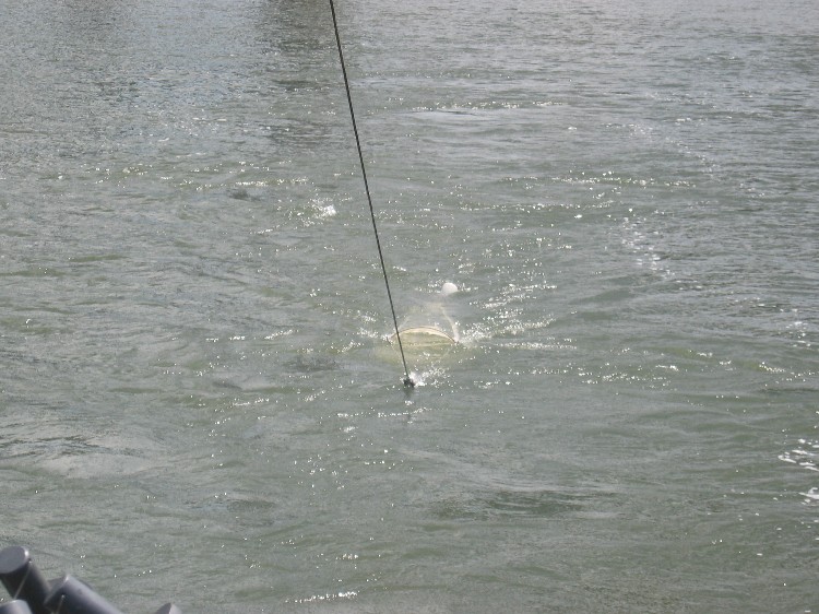
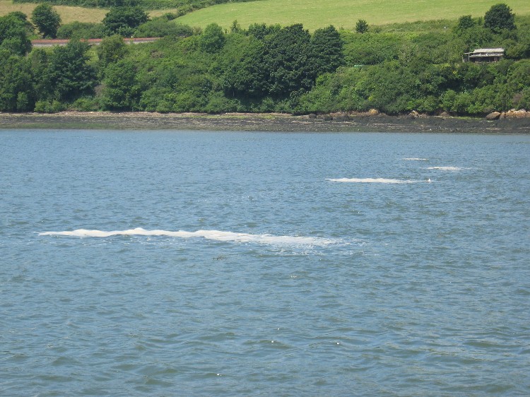
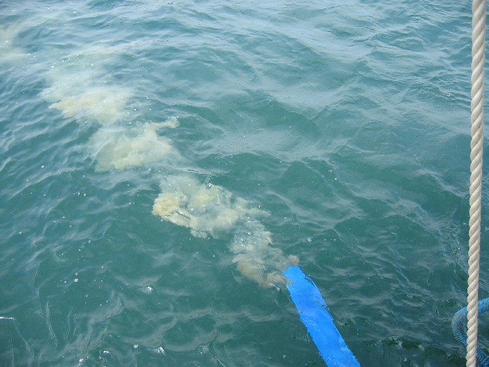
| Figure 46 - Plankton net trawl | Figure 47 - mixing line at the Lynher river, white is oils from organisms foaming at the surface |
The Conway CTD was calibrated with the RIB CTDs before sampling began,
to ensure that the data collected by each vessel could be compared and
valid conclusions drawn for the entire area of estuary sampled.
Below are the
references for the lab procedures which were undertaken to analyse the
samples collected:
Manual chlorophyll, dissolved Phosphate and Silicon:
Parsons T. R. Maita Y. and Lalli C. (1984) “ A manual of chemical and
biological methods for seawater analysis” 173 p. Pergamon.
Dissolved oxygen:
Grasshoff, K., K. Kremling, and M. Ehrhardt. (1999). Methods of seawater analysis. 3rd ed. Wiley-VCH.
Nitrate by Flow injection analysis:
Johnson K. and Petty R.L.(1983) “Determination of nitrate and nitrite in seawater by flow injection analysis”. Limnology and Oceanography 28 1260-1266.
|
|
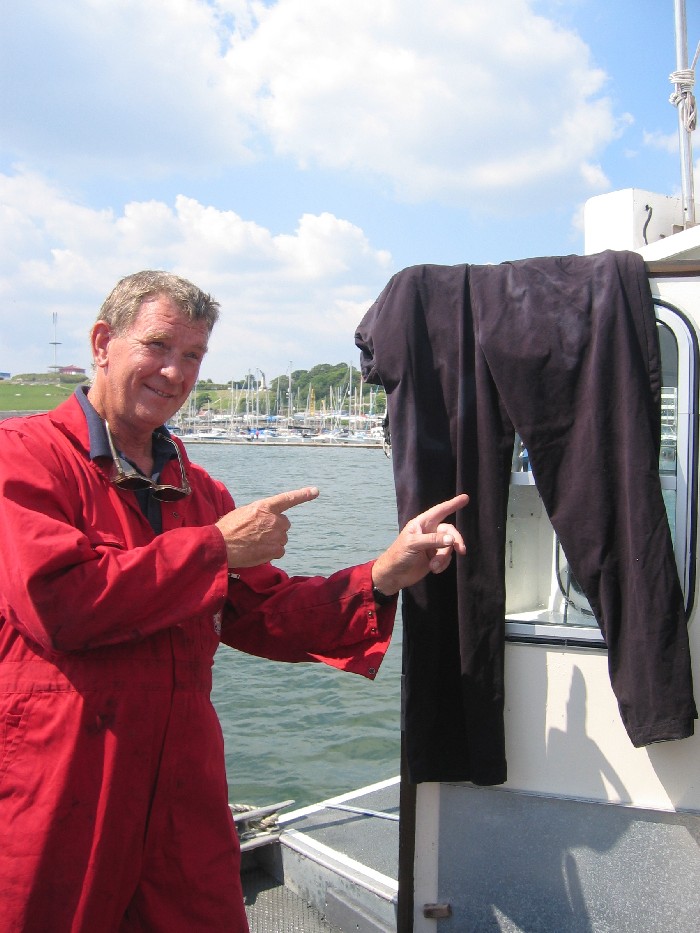
| Figure 48 - Bob had wet pants again!!! |
RESULTS AND ANALYSIS
Plankton
In
estuaries the main factor controlling the abundance and diversity of the
resident plant and animal populations is the salinity gradient, from
freshwater to seawater conditions. As well as salinity, phytoplankton
populations are affected by the amount of available nutrients present in
the system. There is a high input of these nutrients into estuarine
systems from industry, agriculture and domestic sources, so these areas
display high levels of phytoplankton primary production and nutrient
limitation becomes largely irrelevant. This production provides the base
of the food web for other species to populate the system e.g.
zooplankton. The data which our group collected on the Bill Conway
sampling day has been merged with Group 2’s Ribs data for the same day
so that a broader picture of how these changes in salinity and nutrient
availability affect the phytoplankton and zooplankton populations.
 |
 |
| Figure 49 - total zooplankton population numbers | Figure 50 - total phytoplankton population numbers |
At low
salinities on the River Tamar there are high concentrations of nutrients
(Figs. 55 to 58), which decrease as the salinity increases and as you move
seaward the abundance of phytoplankton increases (Fig.50). This is
because the phytoplankton use up these nutrients to reproduce, so from
the phytoplankton abundance graph (Fig. 50) a general increasing trend can
be seen. However this isn’t a perfect correlation as the graph shows, at
a salinity of around 28.8 there were high concentrations of
phytoplankton cells, which suggests a bloom at this location. This
higher cell concentration was also evident in the nitrate concentration
graph (Fig. 56), where at the same salinity an uncharacteristic low
concentration can be seen. This is because the higher number of
phytoplankton in the area needed more available nitrate to reproduce so
the nutrient was used up. This fact is also supported by the number of
zooplankton that were present at that location. The zoo and
phytoplankton display a predator/prey relationship, but there is also
competition for space and in this location the levels of zooplankton are
very low (Fig. 49) because the phytoplankton cell concentration was at a
high level.
 |
 |
| Figure 51 - estuarine phytoplankton diversity | Figure 52 - zooplankton diversity at salinity 20.6 |
Looking at the phytoplankton diversity charts (Figs. 52 to 54) a change in
population structure was evident, at the more saline, seaward end of the
estuary diatoms tended to dominate the community. At a salinity of 28.8
there was further evidence of the ‘bloom’ mentioned above, there was a
change in dominance from diatoms to dinoflagellates, who use nitrate as
there source of nutrition. There was also a change in zooplankton
diversity as the salinity decreases up the river. At a salinity of 35.2
(Fig. 54) there was a varied number of different species present, with
copepods dominating the population. There was a less diverse population
at a salinity of 28.8 (Fig. 53), but no species seemed to dominate the
community. At the last zooplankton trawl, salinity 20.6, the population
was almost entirely dominated by Copepod nauplii with a 98%
share of the community, which may suggest that this species is more
adapted to the freshwater conditions.
 |
 |
| Figure 53 - zooplankton diversity at salinity 28.8 | Figure 54 - zooplankton diversity at salinity 35.2 |
Nutrients
Dissolved phosphate, as shown in Figure 55, displays a typically non-conservative behaviour with variation in the concentrations of dissolved phosphate in respect to the theoretical dilution line (TDL). The reasons for these variations cannot be inferred directly from the estuarine mixing diagram, although hypotheses can be made. In this case variations may be attributed to the alternate variations in the concentration of chlorophyll a, such that when the concentration of chlorophyll a is reduced, the respective concentration of dissolved phosphate is elevated, in respect to the TDL. This pattern is true in salinity range of 0 to 25. In salinities above 25, the dominant process controlling the concentration of dissolved phosphate in the estuary changes, in this area the elevated concentrations of dissolved phosphate could be caused by a sewage outfall located at Henn Point. This may cause elevated concentrations of phosphate due to the fact that both nitrate and silica may be easily removed from the sewage although phosphate is more difficult to remove and so is often discharged in high concentrations into the estuary.
|
|
|
| Figure 55 - phosphate EMD with chlorophyll a concentration overlaid | Figure 56 - nitrate EMD with chlorophyll a concentration overlaid |
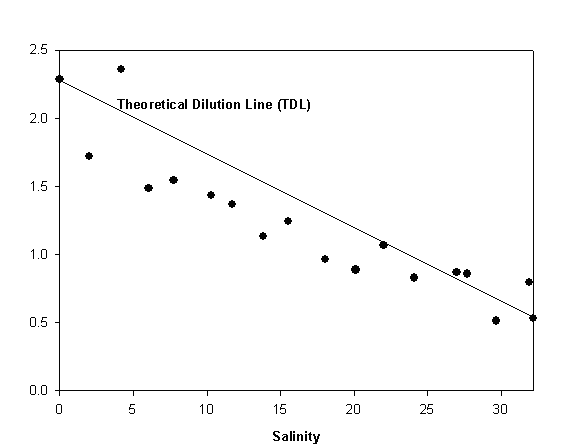
Dissolved nitrate, as shown in Figure 56, displays a consistent removal in the concentration of dissolved nitrate over the whole of the salinity spectrum with a range of 0 to 35, typical of non-conservative behaviour. The reasons for this consistent removal of dissolved nitrate cannot be directly attributed to the estuarine mixing diagrams, although again hypotheses can be made. The consistent removal of dissolved nitrate may be attributed to the removal of this nutrient by phytoplankton because concentrations of phytoplankton remain at a relatively high level throughout the entire salinity range. At the salinity range of 26 to 35 there is a strong removal of dissolved nitrate below the levels of removal observed in the upper estuary, this may be due to the increasing distance of the inputs of dissolved nitrate to these salinities.
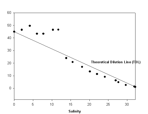
Dissolved silica, as shown in Figure 57, shows non-conservative behaviour throughout the entire estuarine system from zero salinity to salinity 35. The reasons for this behaviour cannot be directly inferred from the mixing diagram, although it may be hypothesized that the reasons for this removal may be attributed to the uptake of dissolved silica by diatoms, which are present in high numbers throughout the entire estuarine system. This phytoplankton species take up high concentrations of dissolved silica for test formation. Dissolved silica may be input into the estuary from mainly riverine and anthropogenic sources such as the runoff of agricultural fertilizers into the estuary that contain high concentrations of dissolved silica.
|
|
|
| Figure 57 - silica EMD with chlorophyll a concentration overlaid | Figure 58 - dissolved oxygen saturation % and chlorophyll a concentration for the estuary |
Dissolved oxygen, as shown in Figure 58, shows low saturations (~100%) in the upper estuary to a salinity of 8, after which the saturation of dissolved oxygen increases to a maximum concentration of 123% at a salinity of 22 and then decreases to ~100% upon reaching the seawater end member. The reasons for this cannot be directly assumed from the figure, although it may be hypothesized that the period in which the estuary was sampled may be after the spring phytoplankton bloom. This would mean that the bacteria in the water column that decompose the dead phytoplankton would use up the dissolved oxygen, known as Biological Oxygen Demand (BOD). Further down the estuary towards the seawater end member the BOD is decreased due to reduced concentrations in chlorophyll a and therefore phytoplankton, causing elevated saturations of dissolved oxygen to occur.
The Richardson Number
The Richardson number
is a measure of the stability of the water column. In Figure 59 the
Richardson number allows the determination of the stability of the water
column of Station 4 in the Narrows, initially on an ebbing tide at
1048GMT and returning to a similar location in the Narrows at Station 4a
on the flooding tide at 1407GMT. This stability may be determined by the
size of the Richardson number such that if Ri<0.25 the water is prone to
mixing because it only takes a low amount of energy to move water from
one depth to another. If Ri>1 then the water is not prone to mixing as a
high amount of energy is required to move water from one depth to
another, so much so that mixing is unlikely to occur and the water is
stable in its arrangement. In Figure 59 the scale only reaches 5,
although many values are greater than 5, because the lines for Ri=0.25
and Ri=1 may be added and variations in stability profiles may then be
viewed more accurately.
|
|
| Figure 59 - comparison of Richardson numbers in respect to depth between stations 4 and 4a |
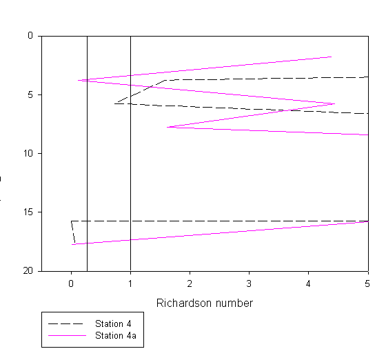
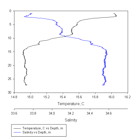
A
comparison of the stability of the water column may be drawn on the
basis of the profiles of Richardson numbers. Such that on the ebbing
tide, Station 4, the water is mostly stable in its arrangement, although
becomes unstable between the depths of 3.5m to 6m and between 15m and
the base of the profile. This may be related to the temperature salinity
profile produced by the CTD at this station, as shown in Figure 60, such
that the water becomes unstable during the thermocline and halocline at a depth of
3.5m to 6m, also the deeper instability may be caused by the variations
in temperature and salinity as shown on the temperature salinity profile
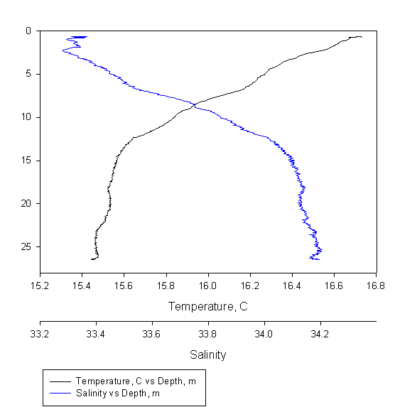
for this station. At station 4a, which was taken on the flooding tide,
the stability profiles vary, such that instability is seen between
depths of 3m and 4m and at a depth of 17m to the base of the profile.
This may again be related to the temperature salinity profile for
station 4a, Figure 61, such that the instability in the upper water
column may be due to alternation of slightly higher and lower salinity
water within this layer. At the deeper depths, the instability may be
caused by the slight variations in both temperature and salinity. The
differences in stability profiles may be associated to the differences
in tidal state in which the profiles were taken.
|
|
|
| Figure 60 - Station 4 CTD Profile | Figure 61 - Station 4a CTD Profile |
ADCP Profiles
STATION 1 -
Transect From Picklecombe
Point to Ramscliff Point
The current velocity along the first transect is relatively slow -
ranging from 0ms-1 to 0.250ms-1. There is an area
to the centre of the velocity profile which shows a water body that is
stationary. This could be caused by the shadow of Plymouth Breakwater.
The velocity direction diagram shows that the vast majority of the water
is moving southward, out of the estuary; this is due to the ebbing tide.
Towards the east of the transect there is an area which shows the water
moving almost in the opposite direction to the main southerly flow. This
is caused by eddying water produced when water has been drawn around the
headland, changing its direction before being turned again by the ebbing
tide.
|
|
|
| Figure 62 - Station 1 Current Velocity Direction | Figure 63 - Station 2 Current Velocity Direction |
STATION 2 - Transect from
Mount Batten Breakwater to Royal Citadel
The velocity of the water is relatively high towards the edge of the
Mount Batten Breakwater, travelling at around 0.3ms-1. The
direction of the water towards Royal Citadel is to the west which could
be due to the input of water from the River Plym and water that has
entered the river area from the Estuary and has changed its direction
with the out going river water. The Backscatter plot shows that there
are high amounts of particulate in the water, particularly in the
centre. This is due to the amount brought in by the River Plym as well
as the marina traffic which stirs up particulate in the water column.
|
|
| Figure 64 - Station 3 Current Velocity Magnitude |
STATION 3 - Transect for the Narrows
- Wilderness Point to Devil's Point
The Direction of the flow in this section of the river is very much
uniform; with all of the water moving with the ebbing tide. The
interesting aspect of this site is the fact that the velocity of the
water is a great deal higher on the eastern side of the channel than the
west. This could be due to bend in the estuary prior to the transect.
Upriver, at station 4, the tidal current continued with a velocity of
0.6m/s directly downriver, with little influence from the West Lakes.
Where 'Looking Glass' protruded near Station 5 (transect to the Navy
Dock), the current reverses and there was slight eddying. At Carew Point
(Station 6), the current velocity was greatest mid-channel, at the
deepest part.
There is evidence of the river input from
the river Lynther towards the south of the channel (left on the plot)
where the direction of the flow is eastward. There is a layer of
sediment to be seen at around 4 metres.
DATA
A full set of data for the
Bill Conway practical can be found at
'group3/conway090705'
BACK TO TOP
QUICK LINKS
|
-
GEOFIELD |
Day 12 -
12.07.05 - 0800-1500GMT
'NATWEST II'
SURVEY PRACTICAL
INTRODUCTION
| WEATHER CONDITIONS | TIDE TIMES | SAMPLING LOCATIONS | INSTRUMENTS USED |
|
Fine and Dry (0/8 cloud); Wind - 0900GMT - S F1 backing SE F3 by 1000GMT Air Temperature - 24°; Sea State - Slight.
|
DEVONPORT (GMT) HW 0909, 4.6m LW 1504, 1.7m |
Outside Plymouth
Breakwater |
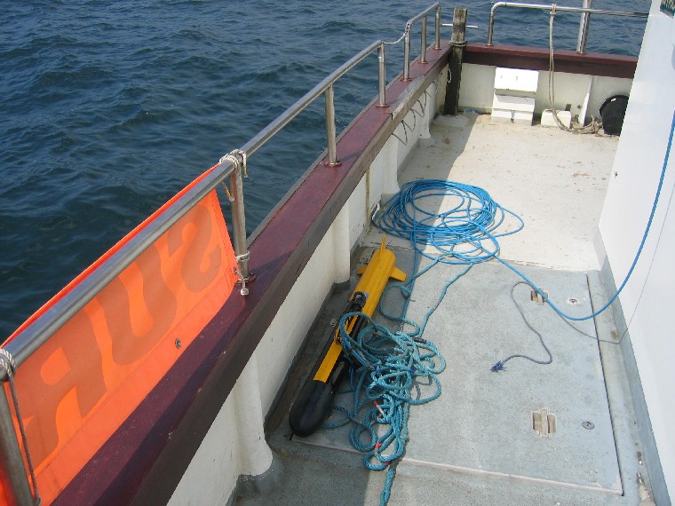
Sidescan Sonar fish |
.jpg)
AIM
The aim of the geophysical survey was to observe the readings from a
sidescan sonar fish towed along a series of transects (created by the group) to
understand how it measures seafloor composition. From this, the aim was
to find varying composition sites within the sampling area and take a
series of grabs to observe the real sediment types corresponding to the
sonar readout. A chart of the sample area was then made to show
understanding of the sonar survey.
METHOD
Calibration of the sidescan equipment was carried out at 08:41 GMT at co-ordinates 50˚20.063N and 004˚11.490W. The ‘fish’ was deployed at 08:55 GMT and transects were taken southwest of the breakwater. Line 1 started at 09:00:24 co-ordinates 50˚20.376N and 004˚10.846W. Line 1 stopped at 09:25:09 co-ordinates 50˚19.589N and 004˚07.994W. Three more consecutive lines were scanned at 100m intervals.
|
|
|
| Figure 66 - Sidescan sonar fish | Figure 67 - Van veen grab |
Once the sidescan data
had been observed three locations were chosen for grabs. These were
chosen to give samples in differing sediment types. Grab 1 was taken at
11:09:12 co-ordinates 50˚20.141N and 004˚10.445W. Grab 2 was taken at
11:31:06 co-ordinates 50˚20.107N and 004˚10.353W. Grab 3 was taken at
11:49:50 co-ordinates 50˚19.899N and 004˚09.225W. Each grab sample was
sieved to determine sediment size, sorting and biological presence. A
fourth grab was taken by recommendation of the staff onboard at 11:56:25
co-ordinates 50˚20.104N and 004˚09.437W.
|
|
|
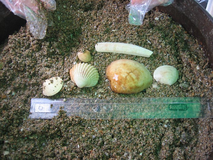
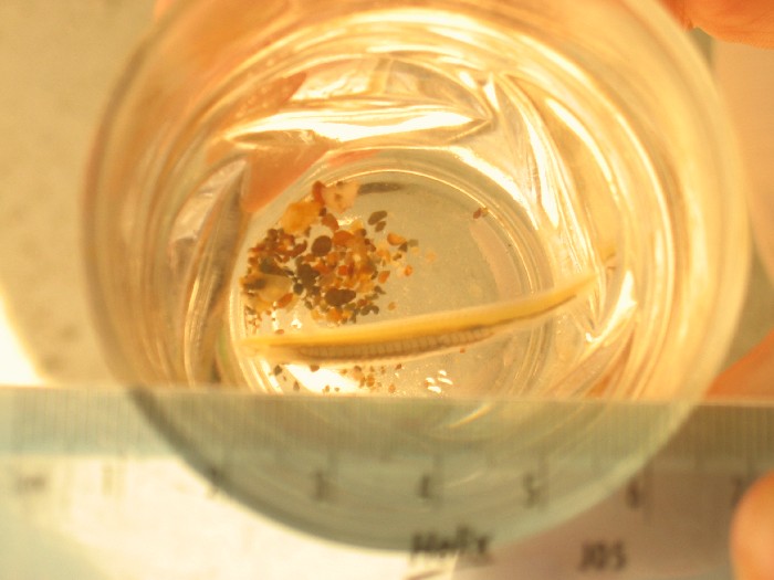
| Figure 68 - sample from grab 1 | Figure 69 - amphixous |
 |
 |
| Figure 70 - discharge of fine sediment from the filter | Figure 71 - another member of staff asleep!!! |
RESULTS AND ANALYSIS
.jpg)
Figure 72 - chart displaying the sediment
types observed by the sidescan
Once the raw data of the 4 transects had been processed and placed in a large graph, the formation of the sea bed from south of Plymouth breakwater to Cawsands Bay in the west can be seen.
The most abundant substance found was sand which can mostly be found within the main channel to the west of Plymouth sound. The far western point of Plymouth sound can be seen as bedrock at 246500, 50500 on the graph. This sand was found to be completely flat, this is due to the high velocity of the water and the fact that the channel has previously been dredged, removing any chance of ripples.
Sand was found with two types of ripple at the breakwater and in Cawsands Bay. The breakwater has sand with parallel ripples formed by tide action; these are parallel due to the movement of water in one plane. Sand in Cawsands Bay has bifurcating ripples caused by wave action.
Grab one, taken within the main channel, brought up very well sorted shell rich gravel. Grab two taken south of the breakwater, found much of the same. Grab 3 failed to sample the sediment. Grab 4 was taken north of the breakwater and found well sorted mud with benthic organisms present. Also an anoxic layer was found at this site.
DATA
A full set of data can be found at Group3/Geophysics120705
Overall Conclusions
From the 30th June to 14th July 2005 Southampton University Oceanography undergraduates surveyed and sampled the river Tamar estuary and surrounding coastal waters. Unfortunately due to adverse weather conditions we were unable to travel further than the breakwater on the offshore boat. As a result of this our data is restricted to within the estuary, although we were fortunate enough to get 300m past the breakwater when on the Nat West II.
Due to the time of year the survey was carried out the end of a spring bloom was evident in the samples collected on all of the estuarine boats (Bonito included as we sampled the estuary). A general trend was observed in the amount of phytoplankton collected at the seaward end being higher than that at the riverine end member. Zooplankton populations correlated with the phytoplankton populations due to their predator prey relationship, a peak being followed by a trough, alternately.
As expected the nutrients followed the trend that they were higher at the riverine end than the seaward end member, this is due to the input from the river and due to heavy rainfall. These high nutrient levels along with previous hot weather could be a cause for high phytoplankton abundance (a mini bloom) thus high zooplankton levels. Non conservative removal of silica was evident this was due to the high diatom numbers dominating the phytoplankton population. All other nutrients behaved conservatively.
The physical properties of the estuary were considered from zero salinity in the upper reaches at Calstock to the Breakwater. In the initial part of the field course most of the physical properties were controlled by the halocline due to the unusually wet and windy conditions creating a more well mixed water column, rather than the expected partially mixed estuary, with a small halocline due to the input of fresher water from a variety of riverine sources including the River Tamar, River Tavy and the River Lynher in the Tamar Estuary and the River Plym in Plymouth Sound. The development of a thermocline was seen after the weather improved somewhat and this lead to differing physical characteristics of the water column that were more controlled by a thermocline rather than halocline. The velocity of the water within the Tamar estuary was seen to increase when travelling around the meanders due to the centrifugal forces that apply; these forces also allowed the setting up of significant eddies in this system, in areas such as Barnpool in the Tamar Estuary and south of the Royal Corinthian Yacht Club in the River Plym, creating both mixing and instability.
AND FINALLY . . .
We would like to say a special thank you to Anthony
and Simon for all they help and hard work over the past two weeks (
offshore boat excluded, see figure 23). We'd also like to thank all the
members of staff and PhDs. A massive shout out to all the boat crews who
made all the hard work seem like fun, especially Bob and his bananas.
BACK TO TOP