


| |
|
|
|
|


![]()
INTRODUCTION
The aim of this investigation was to produce a thorough survey of the physical, chemical and biological characteristics of the Tamar estuary, Plymouth, UK. The data collection and initial analysis was performed from the 30th June through 14th July 2005.
The drowned river valley of the Tamar estuary forms a natural boundary between Devon and Cornwall. Plymouth sits at the mouth of the estuary, which is one of the most researched. The comprehensive understanding of the Tamar is applied to assist the understanding of worldwide estuaries. "An estuary is a semi-enclosed coastal body of water which has a free connection to the open sea and within which sea water is measurably diluted with fresh water derived from land drainage.” Cameron and Pritchard., 1963.
The area of study starts at a depth of 50m offshore to the head of the salt intrusion in the upper reaches of the Tamar estuary. Plymouth sound is formed from the confluence of the main rivers Plym and Tamar. The sound has a maximum width of 6km with a 5km wide mouth. There is a 1nm long breakwater sited at the southerly end of the sound. Flowing from its source, 50 miles north of the city, the River Tamar is the dominant freshwater input into the system. Recorded flow discharges range from 5 to 140m³s-1, with an average of 22m3s-1 (Uncles & Stephens, 1990). The region is mesotidal to macrotidal, partially mixed and flood dominant. The tides ranges from 2.1m in neap tides to 4.7m in spring tides.
The Tamar estuary also consists of three other freshwater inputs, the rivers Tavy, Plym and Lynher. These are all inputs found at the intertidal zone, the domain of mudflats and reed beds. Dredged channels at the mouth direct the majority of flow to the north of Drake's island. Here the channel moves around the eastern side of the Sound until it splits at the breakwater to create the Eastern and Western Channels.
By topography the estuary is classified as a ria. The ria systems entering Plymouth sound (St John’s lake, and parts of the Tavy, Tamar and Lynher), the large bay of the sound, Wembury bay, and the rias of the river Yealm are of international marine importance, due to their wide variety of salinity conditions, sedimentary and reef habitats.
![]()
GEOFIELD- Investigation into geological aspects of the Tamar estuary
Contents
![]() (Click left mouse
button on contents to navigate to point)
(Click left mouse
button on contents to navigate to point)
3. Features of the Region - Antiform, Fault and Cliff face
LOCATION: WEATHER:
Renney Point at Heybrook Bay, Plymouth Cloud cover: 8/8
Easting: 49250 Wind: SW F4
Northing: 49770 Other: Showers
A brief investigation of the form and history of basic geological structures was carried out in the Heybrook Bay area. This is to give an idea of the geology surrounding Tamar estuary. The region is dominated by sedimentary rock deposited between 360 to 400 ka BP (Devonian). This area has since been subjected to changing environmental conditions, resulting in different sediment and rock formations.
Starting at 10:00GMT on Friday July 1st 2005, the survey focused briefly on true dip and strike measurements before considering the history of folding and faulting in the region.
![]()
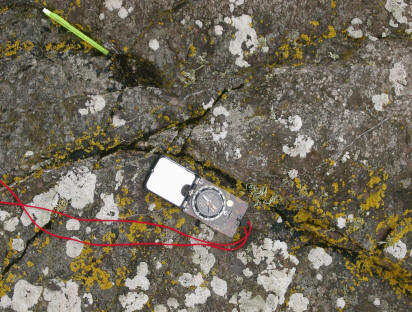
Measurements of dip and strike are made using a compass clinometer (Fig.1). Strike is defined as the horizontal measurement along the rock bed. It is measured by aligning the compass clinometer along the horizontal plane of the rock and reading off the value indicated by a small black arrow. Dip is the angle that a rock bed is tilted away from the horizontal. This is measured by laying the compass clinometer down the angle of the rock face, aligning north, and reading off the angle indicated by the arrow. The direction of strike is found using the right hand rule.
![]()
The group noted several features of geological interest in the area. These included:
· A right-lateral (dextral) fault
· An antiform fold
· A layered sedimentary cliff section
· Numerous fractures
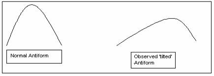
An antiform is a fold in the rock structure in a particular arrangement. A normal antiform is curved smoothly in an inverted ‘u-shaped’ structure. However, the antiform studied in Heybrook Bay was tilted over to one side (Fig.2). This exposed the hinge line (the axis of the fold) allowing us to observe its structure, and make assumptions about its formation. The fold has clearly been pushed into shape by horizontal forcing of some kind. The antiform also has a fault running horizontally across it which must have been caused by a different tectonic event. It is also probable that the fold continues under the beach with an opposite synform structure.
 |
|
| Fig.1 – Compass clinometer and pencil alongside fractures associated with the antiform. (Shows a right lateral fault) | Fig. 2 – A diagram to show the tilted nature of the antiform in Heybrook Bay. |
![]()

Along a direction of 120 o, a fault is present in the rock structure. It can be seen from the current rock arrangement (Fig.3) that there has been movement to the right in each direction by approximately five metres. This is classified as ‘right –lateral’ or ‘dextral’. During a period of stress the region of rock has experienced lateral compression, resulting in pressure and an eventual failure diagonally across the antiform (Fig.4).
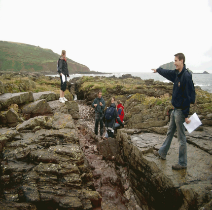

| Fig.3 - Group members stand on the hinge line of an antiform fold in the rocks. In this case a right lateral (dextral) fault has displaced the two halves along a direction of 120o | Fig.4 - A diagram to show the formation of the dextral fault by lateral pressures. As shown, the compression causes weakness and then eventual movement in the diagonal plane.. |
![]()
After the analysis of the various rock structures, an exposed 4 meter section of sedimentary cliff face was studied. The cliff face (Fig.5) had a red colour to it indicating that at the time of formation, oxygen was present in the environment.
The structure of the beds shows how the deposition environment ranges from Sub-aerial to Marine over time. Evidence supporting this conclusion can be seen when moving from the base to the top layers. At the bottom, there are terrestrial riverine deposits, whereas in the higher layers, there are shells.
The first three layers show evidence of mudflows in an era of increased precipitation. This era was probably at the warm climatic optimum (about 8000 years ago) leading to dramatic atmospheric conditions. The North Hemisphere became warmer and more humid as a result of Milankovitch cycles reaching their peak. The cycles, dominated by eccentricity amalgamate to produce warm phases through time. Vegetation was less established at this time meaning that the soil was much less consolidated and therefore more prone to mudslides and mass movement.
|
A layer of fine grain and shell deposits could be human middans. A reddy/brown terrestrial deposit as it is oxidized.
Poorly sorted red/brown layer. Large angular pieces matrix supported. Poorly sorted. There is clay and grit which suggests there has been a slurry flow, slide or slump. There has been some kind of slope failure shown by the eroded material. This was possible due to low vegetation and a period of high precipitation. This layer is more red than the previous layer below, indicating an oxygen rich environment. Poorly sorted and less fine than previously deposited layer. Brown/orange colour. Matrix of fine sediment/clay with a few angular rocks. Poorly sorted with a brown/orange colour. Angular and rounded. Well sorted. Gravelly. In contact/clast supported. Deposition may be by a river as there are rounded deposits. The angular pieces suggest they have not traveled as far as others. Orange colour suggests oxidized. |
Figure 5 – A photograph of the exposed cliff section. |
![]()
![]()
ESTUARY - An investigation into the nutrient, phytoplankton and zooplankton distribution in the Tamar Estuary, Plymouth 02/07/05
Contents
![]() (Click left mouse
button on contents to navigate to point)
(Click left mouse
button on contents to navigate to point)
1. Introduction - Conditions, Richardson Number, Station Location with Map
Physical & Biological Properties - Temperature & salinity vs. depth profiles (stations 1-5), Station 1, Station 2, Station 3, Station 4 & Station 5
Phytoplankton & Zooplankton - Phytoplankton, Zooplankton
Chemical Properties - Nutrients, Nitrate, Phosphate, Silicate
Survey Vessel: Bill Conway
Tides: Neap tide, flooding for duration of survey HW – 0210, 4.5m
1440, 4.51m
LW – 0820, 1.95m
2050, 1.93m
Weather conditions: cloud cover- 8/8, dry although has been rain for last few days.
Sampling: salinity, temperature, depth, [Si], [NO3], [PO4], [O2], phytoplankton, zooplankton
Equipment: CTD, ADCP, plankton net, Niskin bottles and Secchi Disc
The Tamar estuary is joined by many rivers such as the Tamar and the Lynher. These freshwater inputs influence the mixing processes within the estuary and hence its biology and chemistry. This investigation will look into the physical processes involving the concentration of nutrients, chlorophyll and oxygen in order to determine the physical structure of the estuary and how it varies from the upper estuary to the offshore region. The abundance of phytoplankton and zooplankton will also be analysed in order to deduce what could be controlling or limiting primary production in the area. Sampling took place from just inshore of the breakwater, up the river Tamar to the Tamar bridge. In order to get a full overview of the processes influencing the estuary, data from further up the river is required ( from Tamar bridge to Calstock). Data collected on the same day by group 3 was used in order to obtain measurements for the entire estuary over the same tidal and weather conditions.
RIBS
The aim of this boat day was to develop an understanding of how the Tamar estuary acts as a transition zone between the freshwater input and the coastal sea. The small vessels ‘Ocean Adventure’ and ‘Coastal Research’ were used, being shallow draught vessels allowing sampling in areas not accessible to the Bill Conway.
To calculate the earliest time of sufficient water depth for the boat’s draught, secondary port data and a tidal curve were utilized. Our arrival at Calstock (the point of zero salinity at that time) could be no earlier than 0940GMT.
At every two salinity units, samples were taken along the salinity gradient of the River Tamar, with each boat sampling alternate stations. The tide was flooding meaning that samples were taken against the flow of water. The initial sample was taken at Calstock at 1130GMT. At each subsequent station measurements of temperature, salinity, percentage of dissolved oxygen and pH were taken using a T/S probe with digital computer. Water samples were also collected for later chemical analysis. At these sites the 1% light depth (a good indicator of the euphotic zone) was estimated using a Secchi disc. Two samples for oxygen analysis were collected using Niskin bottles at relatively high salinities (18 and 28) in order to minimise contamination by large amounts of suspended sediment. Lugols bottles were used at four locations to give an indication of the phytoplankton along the estuary. Finally, a phytoplankton net with a 50cm diameter was deployed for seven minutes while the rib was stationary at a buoy. At this location the engine was switched off to minimise the disturbance of the sample.
![]()
The Richardson number is used to calculate the stability of the water column, and therefore to assess the mixing that occurs in the estuary. It is important to realize that the relative combinations of stratification and mixing play a crucial role in estuarine dynamics. This is because a stratified fluid consists of a density gradient that will resist the exchange of momentum by the turbulence, and an extra velocity shear is needed to result in any mixing between the layers.
The gradient Richardson number (Ri) is a comparison of the stabilizing forces of the density stratification to the destabilizing influences of the velocity shear.
For Ri > 0 the stratification is stable;
For Ri = 0 the stratification is neutral, and the fluid un-stratified between the two depths;
For Ri < 0 the stratification is unstable.
To obtain the Richardson number the velocity and depth measurements were taken from the ADCP, and CTD readings respectively. The density was calculated by using the temperature and salinity values from the CTD drops.
![]()

Location: Stn1 – Tamar Bridge 50.24.400N, 004.12.203W
Stn 2 – River Lyhner input 50.23.940N, 004.12.489W
Stn 3 – St Johns Lake 50.22.257N, 004.11.120W
Stn 4 – Narrows 50.21.558N, 004.10.154W
Stn 5 – Inshore of Breakwater 50.20.595N, 004.09.913W
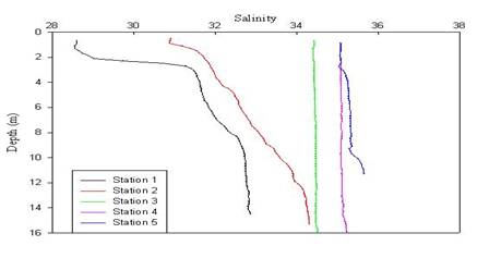
| Fig. 1. Shows positions of each sample station, 1,2,3,4 &5. Click on one of the stations on the map or from the location list to review graphs and data. |
![]()
Physical & Biological Properties
Biology
Fluorometer measurements were used from the CTD as a proxy for reliable chlorophyll measurements. The fluorometer measurements generally show the same trend as chlorophyll for each station down the estuary. At all stations chlorophyll is decreasing with depth, with highest concentrations at the surface. However, it should be noted that only 3 samples were taken down the water column, more samples at more depths would give a better representation of the stratification in the water column.
Temperature & Salinity vs. Depth Profiles
 |
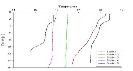 |
| Fig 2. - Salinity vertical profiles at all stations | Fig 3. - Temperature vertical profiles at all stations |
The temperature and salinity reflects the vertical fluctuation in the water column from stations at the head of the estuary to the offshore region (figs 2 and 3 respectively). A distinct halocline and thermocline at stations 1 and 2 can be seen at ~2m depth suggesting fairly stratified waters with warmer, less saline water on the surface and colder more saline water at depth. Moving towards the offshore region there is an increase in the mixing taking place, indicated by the fairly straight vertical lines for stations 3, 4 and 5 which shows a uniformed salinity from surface waters through the water column. This is also reflected in the temperature (fig 3) as at each station the temperature decreases moving further offshore but remains fairly uniform in the vertical profile.
![]()
![]()
Station 1 - Physical & Biological
Station 1 - Physical
The Richardson Number is 12.81, thus showing a stable stratification. This site had the lowest salinity value recorded, 28.61 for the 5 stations sampled. Thus this site was one with the most influence from the river Tamar.
With regard to density there is an evident change in the structure of the water column. At the surface 3 metres there is a rapid increase in density followed by a middle layer between 3-9 metres. Below this layer is the bottom layer after which the density does not change significantly.
As density is primarily affected by temperature and salinity it shows that warmer less saline, riverine water is flowing over the saline intrusion from the sea as it flows northwest up the Tamar. The riverine input data from the ADCP shows that it's also mostly being pushed northwards. This would be caused by the flooding tide, forcing salt water up the estuary. At the surface there is slight southwards trend for flow recorded at the surface, this could be due to the southerly wind that was present on the day.
/Physical/CTD/Processed%20Data/Diagrams/Station%201(density).JPG) |
|
| Figure 3 . Station 1 Density/ Depth profile | Figure 4. Station 1 East-West Transect ADCP recorded data |
Station 1 - Biological
A peak of chlorophyll and flurometer measurements were recorded up to the depth of 3m which correlates with the euphotic zone measured as 3.9metres, then decreases with depth. There is a definite step structure to this graph. As this was the most stratified of all the water columns recorded. Nutrients will mix between the different density waters, being depleted by phytoplankton in the surface, euphotic waters and regenerated in the lower waters. Nutrient concentrations for this site were found to be below the theoretical dilution line, hence being removed from the surface waters.
/Biological/Chlorophyll/Diagrams/Chl%20Station%201.JPG)
Figure 5 Station 1 Fluorometer/ Chlorophyll measurements with depth.
Chlorophyll and Oxygen Depth Profile
Figure 25. Vertical profile of O2 and chlorophyll abundance for station 1.
Within the water column at station 1 on 02-0-05 the chlorophyll abundance ranged from a value of 6.45 at the surface, down to 3.mg/l at a depth of 6m (fig 25), this value then increased again to 4.25 mg/l at 14.4m.
The oxygen values ranged from 102.5 (% saturation) at the surface, down to 111.5 (% saturation) at 14.4m. There is a slight increase in this decline at 6m, the same depth at which the chlorophyll minimum was found.
The decline in chlorophyll readings of the surface waters down to 6m is a result of the light attenuation. At this station the euphotic depth of 3.9m was calculated from the secchi disc depth of 1.3m. This method gives a crude measurement of the depth at which the light can penetrate into the water column, and when looking at this in relation to chlorophyll and oxygen data it is important to consider the margin for error. The Secchi disc measurement relies solely on human observation, and therefore will be susceptible to variations within the results. Although it is important to make sure that the same person takes the measurements each time during the survey, it must also be considered that this measurement may be quite different from that of another person’s observation.
Chlorophyll, and therefore phytoplankton numbers declined through the water column, as less light will reach them. The oxygen levels are increasing down to a depth of 6 metres, and then this increase slows a little, as shown by the steeper gradient on the graph from 6 metres to the deepest reading of 15 metres. This is because the photosynthesis is light limited below the euphotic zone, where visible light does not penetrate. The oxygen levels do not decrease, due to the mixing processes that are occurring within the bottom layer of the estuary. However, it must also be noted that in comparison with the rest of the data set, the value of 115.5 % saturation found at 14.4m does seem to be higher than we would expect. It should be noted that this may be due to a sampling error, or indeed an error during the lab work.
![]()
![]()
Station 2 - Physical & Biological
Station 2 - Physical
Richardson number =1.189, corresponding to a stable stratification. However, in comparison to Station 1 positioned further up the estuary, we can see that the water column although, still stable, may have a higher degree of mixing, this is suggested by the fact that the Ri number for station 2 is considerably lower than station 1 which in turn promotes a higher degree of mixing.
Density (fig 5) shows a fairly constant change in stratification from 1022.0 density units to 1025.0 over the 16 metres sampled. There is not a clear stratification further up the estuary. ADCP (fig. 6) data shows a flooding tide as before, though there is a surface layer of water that appears to be stationary relative to the other water which shows a general trend to be moving northwest. This patch of water was observed on the surface water, and is believed to be because of wind from the hills forcing only the surface water south. The Lynher has also not been found to cause localized perturbations to the salinity gradient when there has not been surface rainfall (Morris et al, 1982).
|
|
 |
|
Figure 6. Station 2 Density/ Depth profile |
Fig 7. Station 2 ADCP profile |
Station 2 - Biological
Station 2 recorded a sloping constant gradient of chlorophyll decreasing with depth. The euphotic zone was measured to be at depth 5.43m. Due to slightly less stratification and more mixing, phytoplankton does not accumulate in the surface waters as in station 1.
/Biological/Chlorophyll/Diagrams/Chl%20station%202.JPG)
Figure 8. Station 2 Fluorometer/ Chlorophyll measurements with depth
Chlorophyll and Oxygen Depth Profile
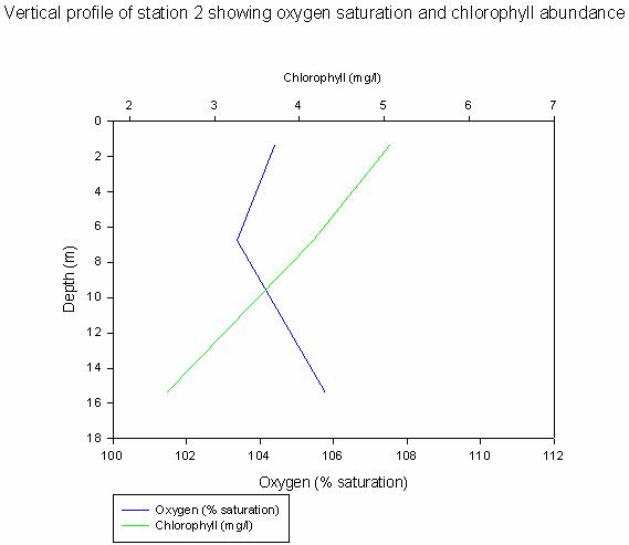
Figure 26. Vertical profile of O2 and chlorophyll abundance for station 2.
Chlorophyll ranges in abundance from 5mg/l at the surface waters, to 2.4 mg/l at 15.8 metres depth (fig 26). This decline is constant throughout the water column as a result of the mixing processes present at this station. As you can see from the temperature-salinity graph for this station (see Fig 1 & 2), the water column is well mixed, without a high degree of stratification.
The oxygen saturation levels decrease from 104.35, to 103.4% saturation at 7 metres depth. At this stage in the water column they then begin to increase at a relatively rapid rate up to 105.8 % saturation at 15.8metres. As with the chlorophyll, these values do not vary greatly throughout the water column,
The chlorophyll abundance declines through the water column due to the light attenuation, limiting the photosynthesis, and therefore the primary production.
The oxygen levels decrease from the surface waters down to 7 metres as a direct result of the decline in phytoplankton numbers, shown by the decrease in chlorophyll. The increase seen at 7m is something that we are unable to account for, and is quite possibly due to an error in either then sampling or the titrations.
![]()
![]()
Station 3 Physical & Biological
Station 3 - Physical
Richardson Number=0.044 Unstable. The change in density of 1025.35 - 1025.15 (fig 7) is not a significant change when compared to the two stations sampled further up the riverine end of the estuary. The salinity and temperature both only change up to 0.2 salinity units and degrees Celsius, respectively which is not hugely significant, this coincides with studies by Morris et al, 1982.
From the ADCP data shown in figure 8 there were eddies recorded here. The eddies are where the water is recorded to be travelling at a slower speed and in a different direction to the modal flow of the flooding tide. This is because the tidal water moving up estuary is moving at a higher speed than the eddies which are moving with the flow. These are important for surface mixing, and also demonstrating the unstable quality of this water column.
/Physical/CTD/Processed%20Data/Diagrams/station%203%20(denisty).JPG) |
 |
| Figure 9. Station 3. Density/ Depth profile | Figure 10. Station 3 ADCP data |
Station 3 - Biological
This water column is well mixed and the chlorophyll measurements are very scattered (fig 11), this could be a product of phytoplankton being mixed throughout the water column. The euphotic zone was measured to be at 11.1metres. Station 4 has a Similar depth and a similar distribution profile of chlorophyll suggesting the mixing processes of these two stations are the same, Richardson number also emphasizes this ( refer to physical section of station 4.)
/Biological/Chlorophyll/Diagrams/Chl%20station%203.JPG)
Figure 11. Station 3 Fluorometer/ Chlorophyll measurements with depth
Chlorophyll and Oxygen Depth Profile

Figure 27. Vertical profile of O2 and chlorophyll abundance for station 3
A different situation is again seen down estuary from that of stations 1 and 2 (fig 27). Here the chlorophyll values range from 2.8mg/l to 2.3 mg/l at 10 metres, and then an increase to 2.8 mg/l at 15 metres. The oxygen saturation increases slightly from surface waters down to 10 metres, ranging from 106.1 % saturation to 106.4 % saturation. Here it then decreases at a more rapid rate to reach 104.55 % saturation at 15 metres depth. At this station the euphotic depth was calculated to be at 11.1m. As you can see from Fig 27 the chlorophyll reaches a minimum at 10 metres, and it is also at this depth that oxygen reaches a maximum. In theory oxygen and chlorophyll should be directly proportional to each other as they are both products of photosynthesis. This again may suggest a degree of error in the accuracy of the euphotic depth calculation. The chlorophyll abundance increases below 10 metres due to the phytoplankton dying, and sinking to the bottom. Mixing of the bottom water will cause levels of chlorophyll to be seen throughout the bottom layer, although levels will be higher as you get closer to the sea bed as the mixing will be more pronounced.
![]()
![]()
Station 4 Physical & Biological
Richardson number= 0.72 unstable. This station, along with station 3, contains an unstable water column and is shown to be well mixed (Fig.10). The density (Fig.9) change is only measured to be 0.2 as with station 3, in other words the density is fairly constant throughout the water column.
This station is at the narrows where water is moving rapidly from west to east, the western side of the narrows has a flow of on average 3m/sec. This velocity is fairly uniform with depth, though when crossing the channel the velocity of water slows and the there is areas which are moving at 0.8m/sec in a southwest direction. This water body could be occurring because of friction and eddies created as the salt water enters this narrow channel. Tidal fronts mark the transitsiton between well stratified shelf water and the well mixed coastal waters (Pinigree et al, 1975)
/Physical/CTD/Processed%20Data/Diagrams/Station%204%20(density).JPG) |
 |
| Figure 12. Station 4 Density/Depth profile | Figure 13. Station ADCP Profile |
 |
At this station we also encountered a tidal front. Although not a scheduled stop, on our way through the narrows a change in the surface waters was noticed where it was thought that the freshwater from the river was coming in contact with the more saline water from the coastal sea. A CTD transect was taken across this area to asses the physical changes. The immediate change in conditions (fig 14) is apparent as two fairly stratified water masses of constant salinities and temperature fluctuate at the time of 10:86.30 when the boat passed the interface of the two water masses. Although the change in temperature was only 0.3°C it is enough to show a variation in the water masses which before the front were fairly constant. This emphasizes the rapid change in the narrows where a large volume of water is moving through a smaller channel. |
| Figure 14 – Shows the tidal front encountered in the narrows | |
Station 4 - Biological
Data shows an extremely well mixed water column with the chlorophyll measurements being very scattered, this could be due to phytoplankton being mixed throughout the water column. The euphotic zone measured to be 11.62 metres, is similar to the depth of station 3 (11.1metres) . As mentioned before they both have a similar distribution profile of chlorophyll, which suggests the mixing processes at these two stations are the same. The Richardson numbers are also relatively similar and so emphasizes the fact ( refer to physical section of the report.).
/Biological/Chlorophyll/Diagrams/Chl%20station%204.JPG) |
| Figure 15. Station 4 Fluorometer/ Chlorophyll measurements with depth |
![]()
![]()
Station 5 Physical & Biological
Station 5 - Physical
Richardson number=0.338. This station was our tidal station and the salinity and temperature figures demonstrate the tidal homogonous properties of this station. This, along with the Richardson number shows a well mixed, unstable water column.
/Physical/CTD/Processed%20Data/Diagrams/station%205(density).JPG) |
 |
| Figure 16. Station 5 Density vs. Depth Profile | Figure 17. Station 5 ADCP Profile |
Station 5 - Biological
/Biological/Chlorophyll/Diagrams/Chl%20Station%205.JPG) |
| Figure 18. Station 5 Fluorometer/ Chlorophyll measurements with depth |
![]()
![]()
Phytoplankton were sampled at five different stations with varying salinities, 16, 27, 28, 32 and 35. 1ml was counted on a cell to determine an average number of species. When counting the phytoplankton chains of diatoms were counted as one single organism. Unfortunately because of this the total number of phytoplankton in the sampled population cannot be determined accurately. Although a very large assumption we can assume that all the chains average the same number of organisms and use this to get an idea of the dominant species of diatom. It should be noted that this method is not entirely accurate and should be an indication of species domination only.
Diatoms were the most abundant of all the phytoplankton at all the stations sampled (figure19 ). Diatoms are the non motile family of phytoplankton and are generally the initial group in the event of a bloom. Their rapid growth rate, and colonies they assume result in the rapid assimilation of the nutrients (Chisholm , 1992). In the ocean this results in a succession of the different phytoplankton groups. The estuary is ideal with the nature of the mixing and the riverine input with a large source of nutrients resulting in a large availability of nutrients. Theoretical dilution lines demonstrate an addition in the lower salinity waters hence a source up river and removal lower down the estuary. This is particularly evident with silica. This emphasizes how diatoms are the dominant class in the stations sampled as they develop the silica frustules. Furthermore, plants need sunlight for photosynthesis, which is affected by the transparency or turbidity of the water or by cloud cover. Water temperature can also have a significant effect on algal production (Kocum et al., 2002).
The maximum total of sampled phytoplankton was found at salnities of 27 and 28. This is highly significant regarding the zooplankton (figure ), as the lowest abundance of sampled zooplankton populations was found at salinity of 29 (need number here). Therefore there is less of a prey effect on these phytoplankton allowing the peak in phytoplankton relative to the other stations.
/Biological/Phytoplankton%20and%20Zooplankton/Diagrams/Phytoplankton.JPG)
Figure 19 Percentage abundance of phytoplankton in sampled surface population at five different salinities in the Plymouth Estuary
/Biological/Phytoplankton%20and%20Zooplankton/Diagrams/Phyto.JPG)
Figure 20 Total number of phytoplankton/m3 at sampled salinities in the Plymouth estuary
Zooplankton samples were taken at 3 different stations at varying salinities along the estuary. Copepods were the clearly dominant species at lower salinities with 63% abundance at salinity of 24 and 28% at a salinity of 29 (fig x and y).
Copepods were also the only species that were found at all sampling stations indicating their tolerant characteristics which allow them to inhabit many different environments. Copepods are also important grazers of the spring diatom bloom (T Kiorboe, 1993), this corresponds to the phytoplankton data where diatoms can be seen to make up the majority of the population.. At the higher salinities of 32 and 35 there are more zooplankton and less phytoplankton thus it could be assumed the zooplankton are feeding off the phytoplankton. Though at salinities of 27 and 28 are where the highest abundance of phytoplankton is found, this correlates with the lowest abundance of zooplankton measured at salinity 29, as three is little zooplankton there is less pressure of predation. The lower abundance of zooplankton represents less of a predation pressure on the phytoplankton allowing a higher abundance
Cairripede nauplii was the second most abundant species at both of the lower salinity sample sites, this is possibly an indication that populations at 24 and 29 salinities are more similar than 29 with 35, this could suggest that there is a point between the salinities of 29 and 35 where the conditions change to favor other organisms. The population sampled at 35 salinity (fig 21), although still containing copepods they only made up 9% of the population, the sample was clearly dominated by Hydrozoans which made up 67%. Hydrozoans perhaps flourish in the more seaward regions of the estuary due to the change in physical conditions; they are filter feeders so rely on particulate organic matter to get their nutrients. The increased mixing in this area of the estuary will create more suspended nutrients that will become available to them. More zooplankton in total was found at the higher salinity of 35 than at either of the other stations with 3.0x10⁹ individuals found per m3 of the sample. At the lower salinity of 24 1.9x10⁹ individuals were counted however the numbers found at the intermediate salinity dropped to 3.6x10⁸. This pattern could suggest that organisms are adapted for either very saline or low saline conditions but struggle more in intermediate salinities. However, the salinities examined in this investigation are all still fairly saline, the lowest being 24 so although there does appear to be a significant difference in the different species found, it is difficult to conclude that this is solely due to salinity. It would be interesting to look at water samples from further up river at much lower salinities in order to get a better comparison.
/Biological/Phytoplankton%20and%20Zooplankton/Diagrams/Zooplankton.JPG)
Figure 21 Total number of zooplankton/m3 at sampled salinities in the Plymouth estuary
![]()
Within estuaries there are the inherent difficulties of drawing generalized conclusions of the physio-chemical properties because of the continuous variability (Morries et al, 1982). This variability can also be biological the relationship between nutrients and plant production in estuaries has been found to be complicated by the natural cycles of the living plants and by climatic and weather conditions; plant growth processes also have a time factor (Neill, 2005). However there are certain means which can be used to gather a general overview of how nutrient distribution changes in the estuary. This method is called the theoretical dilution line, if a nutrient follows the dilution gradient then it’s behaviour is conservative, not having any additions or removal within the estuary (Dyer, 1997). This method was used to analyse nitrate, phosphate and silicate in the Tamar estuary.
/Chemical/Nitrite/Diagrams/Nitrite%20tdl.JPG) Nitrite concentrations generally decrease with increasing salinity (fig
22).
There is a deviation from the TDL at points up river and also in parts of the
lower estuary. Up river at Calstock there was a net gain of nitrite which could
be explained by farm waste run off from two farms adjacent to the sampling
areas. Further down river at the lower estuary (station 3) there is a tertiary
sewage plant which is removing nitrite from the surrounding waters. Thus there
is a net removal of nitrite at salinity of ~34. There is increased mixing
towards the lower estuary (fig 13 and 17)
and a high abundance of phytoplankton which may also account for the
removal of nitrite from the surface waters.
Nitrite concentrations generally decrease with increasing salinity (fig
22).
There is a deviation from the TDL at points up river and also in parts of the
lower estuary. Up river at Calstock there was a net gain of nitrite which could
be explained by farm waste run off from two farms adjacent to the sampling
areas. Further down river at the lower estuary (station 3) there is a tertiary
sewage plant which is removing nitrite from the surrounding waters. Thus there
is a net removal of nitrite at salinity of ~34. There is increased mixing
towards the lower estuary (fig 13 and 17)
and a high abundance of phytoplankton which may also account for the
removal of nitrite from the surface waters.
Fig 22 Theoretical dilution line of nitrite in the Tamar
However limitations of the theoretical dilution line method can not be ignored. The small variation either side of the theoretical dilution line could also be explained by the changes in physical and physiochemical properties. Morris et al, 1982, have found many properties ignored by the theoretical dilution line to be of great importance when studying nutrients in an estuary.
/Chemical/Phosphate/Diagrams/phosphate%20tdl.JPG)
Phosphate concentration decreases with increasing salinity (fig 23) however there is more variance from the TDL which suggests conservative behavior. There is a net loss of phosphate in the upper regions of the River Tamar which can be credited to biological removal via phytoplankton uptake. The net gain of phosphate in the lower estuary was not expected, however can possibly be explained by the presence of the sewage works at station 3. Although the plant removes nitrite and silica it does not have an efficient method of removing phosphate. The lack of silica and nitrite in the water will inhibit phytoplankton growth thus phosphate uptake will decrease thus increasing phosphate concentrations in the surrounding water. This accumulation of phosphate may also be due to the presence of St Johns Lake. The lower estuary generally has regular mixing but the presence of the mud flats mean that water masses are temporarily isolated from the main oscillatory tidal streams which causes re-entrainment and fronts of high static stability thus the retaining of nutrients such as phosphate.
Fig 23 theoretical dilution line of phosphate
/Chemical/Silicon/Diagrams/Silicon%20tdl.JPG)
The Silica concentrations (Fig 24) also decrease with increasing salinity, however it does not follow the same pattern as phosphate as initially expected. The presence of the two farms near to the sampling areas explains the differences in the upper stations of the river, silica concentrations rise (net gain) due to farm waste run off thus increasing phytoplankton growth which in turn increases phosphate uptake by phytoplankton. Lieberg’s law of minimum( Lieberg, 1840) shows that the addition of a single fertilizer will increase crop yield if other nutrients are non limiting, interpretation of this indicates the excess of silica to be the single ‘fertilizer’ that is most important to diatoms when considering this law. The excess of silicate with the other nutrients allows the diatoms to bloom, diatoms being the only group of phytoplankton to assimilate silicate for cell walls, frustules. The net removal of silica can again be credited to non-biological removal by the sewage works. However at higher salinities there is a net removal of silica, phytoplankton analysis showed diatoms to be the dominant phylum in the population at this point, this could explain the silicate removal, and as the silicate is removed more the phytoplankton populations decrease, as seen at the higher salinities of 32 and 35 (fig 19)
Fig 24 theoretical dilution line of silica
![]()
![]()
GEOPHYSICAL - Investigation into estuary bed formation relating to estuarine flow
Contents
![]() (Click left mouse
button on contents to navigate to point)
(Click left mouse
button on contents to navigate to point)
2. Results & Discussion - Map of surveyed area, ADCP profile 1 & ADCP profile 2
NAT WEST 2 – GEOPHYSICS 05/07/05
The aim of this practical was to utilize sidescan sonar and take sea bed samples using the grab. In order to help relate this data to that already gathered, and further enhance knowledge of other studied stations, data collection was centered around the ADCP and CTD stations investigated by the group on 02/07/05 aboard Bill Conway near the Lynher confluence. Conditions were replicated (ie: same tidal period) .This would allow the group to make interpretations on features found at the study sites and produce a trackplot map of the selected region..
Timetable of the day (BST)
09:15 – Leave Mayflower Marina
09:30 – Decide not to travel out to the Scylla due to weather conditions
09:58 – Begin Jennycliff Bay survey (to familiarise with sidescan sonar techniques and check equipment)
(10:33 – End Survey
10:46 – Grab taken Jennycliff
11:38 – Redploy sidescan in region of narrows and begin a transect moving upriver
11:50 – Transect across Rubble bank
12:45 – Reach Tamar bridge and recover sidescan
12:58 – Begin taking 3 Grabs moving downstream
14:04 – Sidescan redeployed and survey of R.Lynher begins
14:49 – Survey ends and begin returning downstream
15:28 – Grab taken on Rubble bank
15:57 – Return to Mayflower Marina. Hydrophone data collected
Notes on the sidescan data interpretation method:
 Fig
1
Fig
1
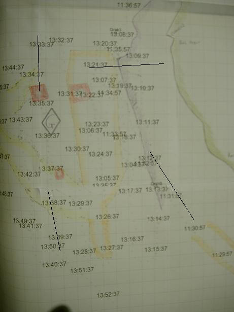
The sidescan sonar data gives the ability to measure depth and slant range. This allows the distance of any features from the path of the boat to be calculated using pythagoras (Fig 1). By using stored navigational data from the ships GPS, a track plot can be produced for the path of the ship over the survey area. On the same plot any features on the seabed can be mapped using the Pythagoras and a scale conversion between the sidescan scroll data and the track plot. In our case this was 1:0.25 or 4:1.

Fig.2 Sidescan sonar trackplot of surveyed region
![]()

* Fig.3 Map showing area surveyed by the side scan sonar, with the position of both the 1st and 2nd ADCP data taken from the Bill Conway. Click on 1 or 2 to review graphs and data.
![]()

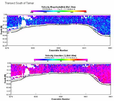
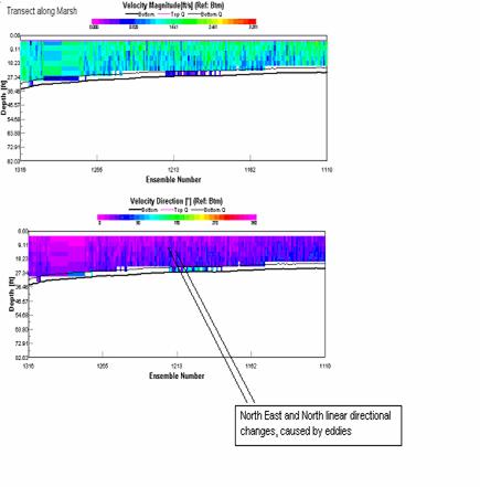
The transect, crossing the River Lyhner is well mixed in comparison to transect 2. This is due to the smaller volume of freshwater input from the Lyhner compared to the Tamar. There is a deep stationary water body from the flooding tide (fig.4) . A water body is likely to be of low velocity or stationary due to the friction from moving round the bend into the Lyhner. A frictional increase also results from shallowing bathymetry. This reduces current speed and can promote rotational currents further assisting the fine grained sediment deposition (Pingree and Maddock, 1985). This correlates with the deposits shown on the sidescan sonar trackplot (Fig. 2) which are classic fine grained river deposits (clays). Deposition has occured in this region of slacker current. The Ri (Richardson Number) number here was found to be 1.88 This refers to non-turbulent flow confirming the depositional environment observed. The water body moving in a southerly direction (Fig.4) is most likely attributable to the wind strength experienced.
|
Fig.4 ADCP North/South Transect of the River Lyhner. |
The spatial accuracy of our trackplot sidescan data was validated by cross referencing with Admiralty charts.
![]()
![]()
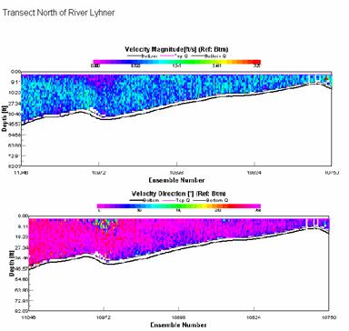
 Due
to the high freshwater input from the Tamar (in comparison to the Lyhner)more
stratification is expected at this second transect. The flow velocity is also
greater, this represents conditions of higher energy. Higher energy conditions
are able to support coarser sediments in suspension. These coarser sediments
become separated from suspension in the flow at slacker periods of the tidal
cycle and settle at the bottom. More specifically, in this region of the Tamar,
Uncles et al. 1984 from Dyer, 1997 identified a net seaward sediment
movement in the main channel with a weaker landward movement in shallower
regions. Three regions of coarser grained sediment (and consequently higher
energy enivroments) were found down the central channel of the Tamar. Material
retrieved from Grab 3 was a clay deposit covered in a small layer of larger
sediment of gravel and sand. Visual analysis of this grab showed slight ripple
bed formation on the surface indicating influence from the flow. The sidescan data shows several
regions with light and dark streaks (ephemeral sediment streaks shown in Fig. 6)
showing coarser sediment randomly dispersed over a
finer sediment due to high turbulent flows. The Ri number
(Richardson Number) in the middle of the channel
equated to 0.044 confirming turbulent flow and mixing. Moving eastwards along
the transect;
velocity increases and there are signs of rotational flow highlighted by a change in
direction of flow in the ADCP data. This concurs with two eddy bedform features
found by the sidescan sonar and shown on Fig.2. Incidentally, the tidal diamond gives an estimated speed of
0.6knts in a 336o direction for the region, supporting the
accuracy of the ADCP which reads an average of 0.6knts.
Due
to the high freshwater input from the Tamar (in comparison to the Lyhner)more
stratification is expected at this second transect. The flow velocity is also
greater, this represents conditions of higher energy. Higher energy conditions
are able to support coarser sediments in suspension. These coarser sediments
become separated from suspension in the flow at slacker periods of the tidal
cycle and settle at the bottom. More specifically, in this region of the Tamar,
Uncles et al. 1984 from Dyer, 1997 identified a net seaward sediment
movement in the main channel with a weaker landward movement in shallower
regions. Three regions of coarser grained sediment (and consequently higher
energy enivroments) were found down the central channel of the Tamar. Material
retrieved from Grab 3 was a clay deposit covered in a small layer of larger
sediment of gravel and sand. Visual analysis of this grab showed slight ripple
bed formation on the surface indicating influence from the flow. The sidescan data shows several
regions with light and dark streaks (ephemeral sediment streaks shown in Fig. 6)
showing coarser sediment randomly dispersed over a
finer sediment due to high turbulent flows. The Ri number
(Richardson Number) in the middle of the channel
equated to 0.044 confirming turbulent flow and mixing. Moving eastwards along
the transect;
velocity increases and there are signs of rotational flow highlighted by a change in
direction of flow in the ADCP data. This concurs with two eddy bedform features
found by the sidescan sonar and shown on Fig.2. Incidentally, the tidal diamond gives an estimated speed of
0.6knts in a 336o direction for the region, supporting the
accuracy of the ADCP which reads an average of 0.6knts.
| Fig.5. ADCP Transect of the Tamar River, North of the River Lyhner. |

Fig. 6. Side sonar map of ephemeral sediment streaks.
![]()
![]()
Contents
2. Results and Discussion - Station 2, Station 3, Station4 and Station 5
The survey was carried out on 12 July 2005 during spring tides, while the tide was ebbing.

(Fig. 1)– Temperature, Salinity and fluorescence with depth at Station 1
The temperature profile at the most landward station showed a small change in temperature down the water column (Fig 1) in comparison to the stations offshore. This is expected in coastal regions where depth decreases and freshwater inputs increase. In these high energy environments a well-mixed turbulent water column is the norm (Pinigree et al, 1975). A small temperature rise near the surface may be accounted for by the diurnal thermocline that we expect to see at this time of year. The ‘front’ or location where the coastal water meets the offshore water, became more apparent in the following stations. The water at station 1 was unstable, as the stabilizing force of density has been overcome by the destabilizing force of tide which increases into shallower depths where the energy is focused. For both silicate and phosphate, the graph shows that there was a very minimal change throughout the water column. The results for oxygen have shown that there was a small increase with depth, however we have to allow for the limit of detection which is 2%. All the profiles for nutrients, oxygen, temperature and salinity have supported our expectations that inshore regions are well mixed due to increased energy and high turbulence from coastal interaction. The euphotic depth at this station was measured at 15m, using the secchi disc. This shows that more than 1% of the surface light reached the sea bed, as the depth was only 10m.
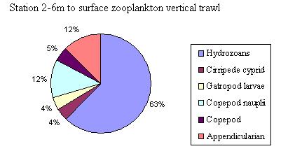
Fluorescence is used to measure chlorophyll, thus phytoplankton. The CTD shows fluorescence increased with depth from 0.3 volts at surface waters, to 2.8 volts at 8 meters. This pattern is also repeated in the phytoplankton counts. At surface they were counted at 160000cells/l and 425000cells/l at 8.6 metres. This is expected during the summer as the mixed layer deepens. Nutrients are less available at the surface as a result of the decreased winds, which in turn decreased the turbulence in the upper layer, during these months. Therefore there were less nutrients for the phytoplankton to assimilate so growth was limited at the surface layers. At this station there was no fluorescence maximum as the depth of the water column was less than the estimated euphotic layer. The groups of phytoplankton found at this station at both depths were diatoms. In a well mixed environment diatoms dominate (Pemberton et al, 2004). The average backscatter for this station was found to be fairly homogenous because of this only one trawl was taken, from the lowest depth to the surface. The sampled population was found to be dominated by hydrozoans, jellyfish. The only meroplankton found in this sample were Gastropod larvae and Cirripede cyprid making up only 9% of the total population sampled (Fig. 2)
Fig. 2

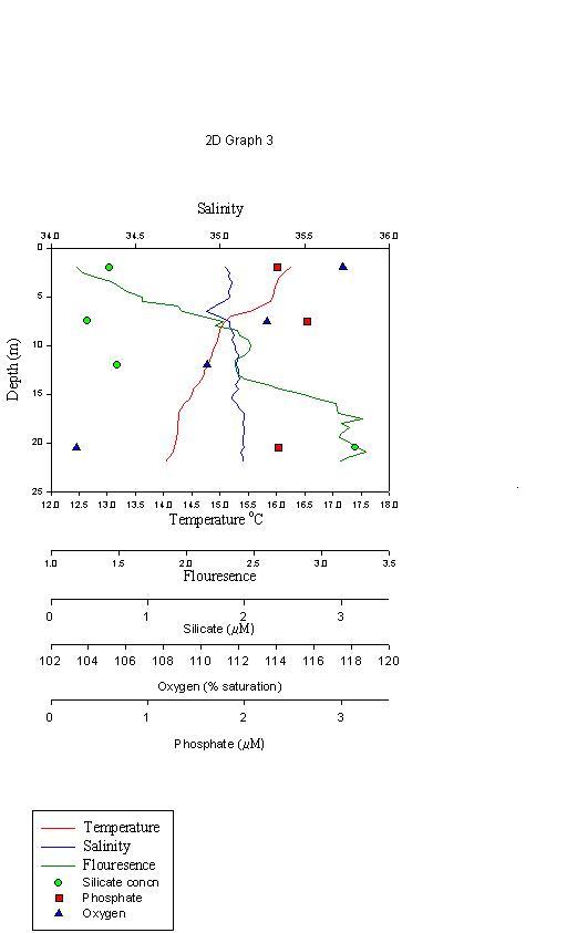
(Fig. 3) above - Temperature, Salinity and fluorescence with depth at Station 2
Slightly further offshore at station 3 we can see that there was a more pronounced thermocline at 10 metres. The water column was therefore more stratified, and more stable. As you move offshore tidal energy decreases, and mixing is reduced. This results in a deeper mixed layer depth.
Fluorescence was shown to decrease with depth. Phytoplankton counts were found to be fairly similar, 190000cells/l and 135000cells/l at surface and 15.58m respectively. This does not agree with the fluorescence though counts can be less accurate due to sampling error. Therefore fluorescence is used as a more accurate parameter. The phytoplankton increased at depth as the nutrients at the bottom of the thermocline are mixed up and could then be utilized by the phytoplankton. Therefore phytoplankton were not limited by nutrients at depth, as they were at the surface layers. Nutrients increase until the euphotic depth when light levels become the major limiting factor to productivity. Using the secchi depth, the euphotic depth was estimated at 14.4m. Using (Fig. 3) we can determine that the euphotic depth corresponded with the fluorescence maximum, both having been at approximately 14.4m, after which fluorescence decreases as phytoplankton become limited by light. The dominant group in the phytoplankton group was diatoms, which utilize silicate to build their cell walls, this correlated with the silicate concentration which also decreases with depth. It has been found that in the frontal region there is expected to be a high phytoplankton community. This is a mixed, recently stabilized, layer because of the high combination of nutrients and shallow mixed upper layer allowing rapid growth of phytoplankton (Pinigree et al, 1975)
(Fig. 4) shows the vertical profiles at station 4 on 12-07-2005
The thermocline was again more pronounced than the previous station (Fig. 4). The concept of less tidal energy causing more stratification further offshore is enforced. The thermocline at station 4 was at 6-8 m. In the peak summer months, it is expected to be nearer 20 m. This may be a sign that the ‘front’ where the two water bodies interact has been found. Phosphate appeared to increase by 0.2 µM just below the thermocline, where the mixed layer may hold more nutrients. It was considered a relevant increase because the amount was more significant than the detection limits of phosphate at 0.03 µM. Silicon doesn’t follow the same pattern however, it increased below the thermocline and reached a peak at the same point as the fluorescence maximum, . Productivity was expected to be high below the mixed layer depth where winter mixed nutrients are more available. Fluorescence showed this with a peak at 18m, though like other stations phytoplankton counts did not correlate with this. A higher concentration of silicate at depth showed why there are lots of diatoms here, and this also could be a product of dying diatoms having fallen through the water column and increased silicon levels at depth. The phytoplankton community at this station had different dominating groups with depth. This could be because of different adaptations to different light levels. There is a trough of zooplankton concentration recorded from backscatter at the depths of approximately 12m, this is correlated with a peak in fluorescence found at 12.1m. Phytoplankton had less of a predator pressure here.


(Fig. 5) – Shows vertical profiles at station 5 12/07/05
Having traveled a total of 6 nautical miles from the coast of Whitsand Bay, the temperature profile clearly showed a very strong thermocline (Fig. 5), at approximately 20m, which is the expected depth for this feature at this time of year. The total range is 4.5°C from surface waters down to a depth of 32.5m. This station was far enough offshore to fully simulate the typical water column of an open ocean. The profile was very stable, and stratified and there was little tidal forcing. The results collected would suggest that this region is no longer influenced by the coastal waters, and oceanic processes are dominant.
The silicon profile seen at station 4 was again replicated here, perhaps inferring the same processes of pelagic diatoms, which die and settle through the water column, giving rise to increased silicon with depth. Phosphate did not show any obvious variation with depth, which is unexpected with such apparent stratification. We would expect a decrease between the surface and the euphotic depth, which was calculated at 21m, resulting from biological uptake. Cross-referencing with the silicon profile it can be assumed that the phytoplankton populations are diatom dominated, as silicon is used and the phosphate does not seem to have been. Once again the fluorescence maximum occurs at the estimated euphotic depth. The fluorescence increases until this depth where light levels are minimal, after which primary production cannot take place. No oxygen was sampled at this station, as we had limited oxygen bottles on-board.
The phytoplankton counts showed surface numbers of 190,000 cells/l (Fig **), which decreased to 95,000 at 13m, and then increased again to a peak of 360,000 at 20.7m, this being close to the euphotic depth of 21m. The numbers then decreased down to 105,000 cells/l at 33.6m. At 21-19m a zooplankton net was taken as from the ADCP there was a peak of backscatter. The base of the euphotic layer was measured to be at 21metres depth. The base of the euphotic zone is where there is mixing up of nutrients and light balance allowing a peak in phytoplankton. This peak of phytoplankton allowed the predator, zooplankton, to prey on them hence a peak in zooplankton. At 12-10m a low value for back scatter was measured (Fig. 6, ADCP for station 5-below), so a zooplankton sample was taken here to ascertain what classes if any were here.
Fig. 6
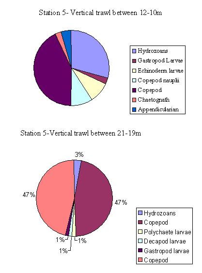
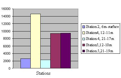
Fig. 7 Station 5 Nitrite concentrations

![]() Temperature
oC
Temperature
oC
![]() Nitrite
Concentrations
Nitrite
Concentrations
Station 5 was the only station to record concentration above the detection limit Fig. 7. Station 5 will have more nutrients because of the regeneration at depth of nitrates from the surface layers. It is highly significant that nitrite is depleted as according to the redfield ratio phytoplankton assimilate it at 16 molecules to every phosphate molecule. This is why nitrite is non detectable at many depths in comparison to phosphate.
Chlorophyll Concentrations
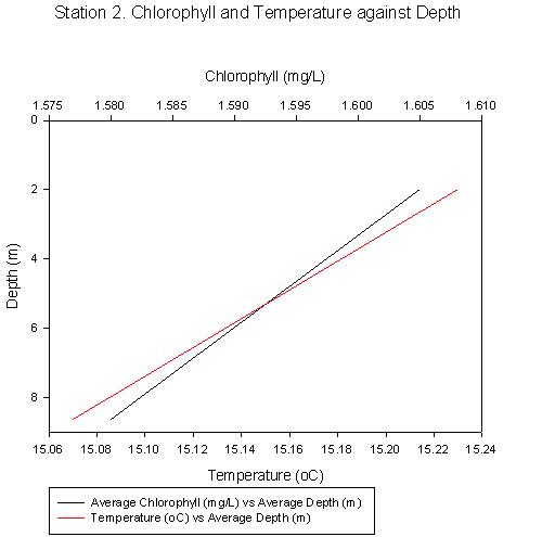
Fig. 1
In this well mixed water column nutrients are consistent through the vertical profile hence primary productivity is linear with depth (Fig. 1). The theoretical euphotic depth is greater than the true depth, and so light is not a limiting factor. The difference in chlorophyll with depth is not large and the limits of detection reduce this difference to almost zero. This enforces the idea that chlorophyll follows the nutrient profile.
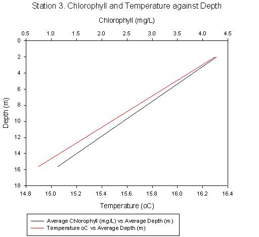
Fig. 2
There is a higher chlorophyll concentration (Fig. 2), which varies a significant amount more with depth than at the previous station. This is due to suspended sediment limiting light in coastal regions. Generally nutrients are the limiting factor in the offshore region, however at this time of year, during the spring bloom, the nutrients are available, plentiful and no longer limiting. This station is still in the well mixed tidal dominated region therefore nutrients are distributed evenly throughout the water column.
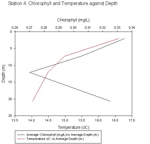
Fig. 3
This station is located in the region of mixed coastal and offshore waters (Fig. 3). This scale shows only 0.1 mg/L variation in chlorophyll and so is slightly misleading. The variation is within detection limits and so chlorophyll can be assumed to follow the same pattern as station 2 where chlorophyll is dependant on the nutrient profile.
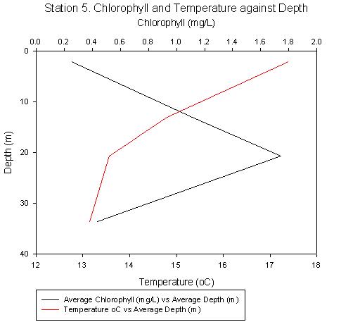
Fig. 4
This station is 6nm from the coast and demonstrates a standard oceanic profile (Fig. 4). Chlorophyll increases with depth until the estimated euphotic zone of 21m, calculated using the Secchi disc measurements. Below this depth, the absence of light does not allow for any primary production.
PLYMOUTH - Concluding Observations
After looking at the different areas of the Tamar Estuary it is apparent that the chemical, physical and biological variances act to produce a dynamic, changing environment. Data has shown it to be a partially mixed, flood dominant estuary. The greatest changes in salinity are found up river as the area is most influenced by physical factors such as rainfall, land and agricultural runoff.
Further downriver in the upper estuary, tidal factors begin to affect the conditions as freshwater inputs come into contact with more saline waters. This causes high stratification with the biological removal or addition of nutrients. The flora and fauna in this region are light limited due to suspended sediment in the water column. The lower estuary is again affected by the two water masses, but is influenced more by the tides rather than the river input. Although sediment is transported down river into the estuary, the flood tide is much stronger than the ebb tide so sediment is transported landwards again.
Moving into the offshore region, rather than being light limited, the area is nutrient limited due to the increased mixing. Phytoplankton are found to be most abundant at the base of the thermocline where nutrients accumulate.
The form of an estuary is constantly altered by deposition and erosion of sediment, over time its dynamics and therefore the species inhabiting the estuary are in a constant state of change.
1. Tidal Mixing in the Channel Isles Region Derived from the Results of Remote Sensing and Measurements at sea. R.D.
Pingree, G. T. Mardell and Linda Maddock (1984)
2. Rotary currents and residual circulation around banks and islands. R. D. Pingree and Linda Maddock (1985)
3. The influence of water body characteristics on
phytoplankton diversity and production in the Celtic Sea, 2004,
Continental Shelf
Research, Volume 24, Issue 17, Pages 2011-2028
Pemberton, K., Rees, A. P., Miller, P. I., Raine, R. & Joint, I.
4. Primary Productivity and Biogeochemical Cycles in the Sea. Chisholm, S.W., 1992. Phytoplankton size. In: Falkowski, P.,
Woodhead, A.D. (Eds.), Plenum Press, New York.
5. Die Organiche Chemi in Ihrer Anwendung Auf Agrikultur Und Physiologie (Organic Chemistry in Its Applications to
Agriculture and Physiology). Liebig, J.V., 1840.
6. A method to determine which nutrient is limiting for plant growth in estuarine waters—at any salinity, Neill, M., 2005, Marine
Pollution Bulletin, In Press, Corrected Proof.
7. Estuarine, Coastal and Shelf Science, Morris, A. W., Bale, A. J. & Howland, R. J. M., 1982, 14, 649-661.
8. Estuaries, A Physical Introduction, 2nd Edition, K.R.Dyer, 1997


Nat west Bill Conway Bonito

From left to right: Alexandra Nichol, Rachel Gibson, Jamie Holmes, Isaac Jordan-Rowell, Ruth Henderson, James Trimmer, Joe Allan and Katie Evans not present.
www.shallowsurvey.com/cds.cfm - Published fly-through and data sets of the Plymouth estuary.
www.metoffice.co.uk - live meteorological data
www.ndbc.noaa.gov - Buoy data for coastal waters.
![]()
/Physical/CTD/Processed%20Data/Diagrams/Station%202(density).JPG)