


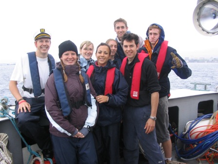
From Left to Right:
Robbie "El Capitano" Smith, Rosalind "Alcoholic" Pidcock, Kelly "Bruiser" Lovegrove, Asha Jones,
Helen Needham, Donald " The Damager" Scott, Steve "The Suppressor" Cundy, Joey "Jim" Morris.
|
|
|
|
|
|
|
From Left to Right: Robbie "El Capitano" Smith, Rosalind "Alcoholic" Pidcock, Kelly "Bruiser" Lovegrove, Asha Jones, Helen Needham, Donald " The Damager" Scott, Steve "The Suppressor" Cundy, Joey "Jim" Morris. |
|
Introduction
Welcome to Plymouth 2005.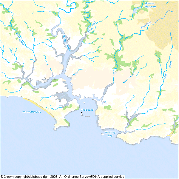
During the field course, water samples will be collected from the upper reaches of the Tamar estuary, through to Plymouth sound and offshore to a depth of 70m to involve riverine, estuarine and offshore environments. The water samples that are to be collected will be used for the analysis of, nutrient concentration, oxygen concentration, fluorescence, chlorophyll, zooplankton abundance and species composition at varying depths within the water column.
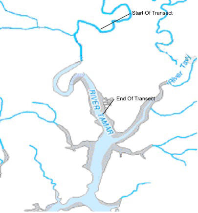
The Tamar estuary, see figure 1, fed by the Rivers Lynher and Tavy, is a partially mixed, mesotidal / macrotidal estuary which travels through the narrows and into Plymouth Sound. The estuary forms a natural boundary between Devon and Cornwall, it is a drowned river valley which stretches for 31.7Km (Tatersall et al.,2003). This drowned river valley is surrounded by intertidal mudflats and reed beds and is considered to be an area of special conservation. The central estuary channel is dredged to accommodate large Naval and commercial ships that frequently use the estuary. Plymouth Sound is protected from the currents and swell of the Atlantic Ocean by a 3km breakwater.
The aim of the survey programme is to investigate the inter-relationship between physical, chemical and biological parameters along the full salinity range 0 – 35.
Figure 1 - Map of Plymouth Sound
This website is a preliminary presentation our results collected over the 2 week period. Water sampling was undertaken on four days on four different vessels. Local geology was investigated around Renney Point.
The main object of visiting Heybrook Bay was to distinguish between fractures and fault lines found on the bedding off the area of Renney Point. Using compass clinometers the dip and strike of the rocky out-crops was measured.
The wave cut platform
This wave cut platform shows detail of known events over geological time.
Figure 2 shows the five different layers which represent the different climate conditions at the time of formation.
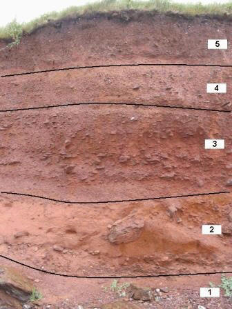
The uppermost layer (5) contained lots of marine, shell fragments and soil was present below the grass. This layer was formed during the Holocene when this area was submerged due to sea level rise resulting from the end of the last ice age.
The forth layer (4) was a fine clay matrix with a small amount of pebbles. The colour was a lighter red to brown colour showing that it was less oxidised in comparison to layer 5. This layer was formed during the climatic maximum when the earth was closest to the sun due to the eccentricity of the earth’s orbit and the precession (wobbling) of the earth on its axis. The proximity to the sun of the northern hemisphere at this time meant that the glaciers reaching down to the Midlands started to melt and released a vast amount of water into the atmosphere. The large amount of water in an environment where there was very little vegetation to stabilise the earth, resulted in frequent mudflows. As the rain falls became more frequent and heavy the loose soil washed away and was deposited further downstream. The knowledge of this time period corresponds well with the evidence of the layer which contained rounded pebbles within a sediment matrix.
Layer three (3) contained flat, layered angular stones in a coarser, with respect to the previous layers, gravel and sediment matrix. The angular stones show that the layer was formed terrestrially and laid down over a long period of time so that a matrix could be built up around the particles.
The second layer (2) was a bright orange colour which indicates that the sediment is highly oxidised as in layer 4. There were a small number of pebbles and a large amount of large angular rocks. This layer was probably formed above sea level on dry land as the stones are angular and there is no evidence in the layer of marine life.
Figure 2 - Shows Typical Cliff Face at Renney Point.
The bottom layer (1) has many small pebbles, similar in number to layer 3 some of which were angular, but most were well rounded in a clay-like matrix. This layer is the oldest and was formed when the area was above sea level. The angularity of the stones indicates that the stones didn’t travel far before being incorporated into the sediment.
01/07/05
Aims and Objectives of boat practical :
Overview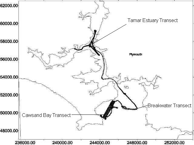
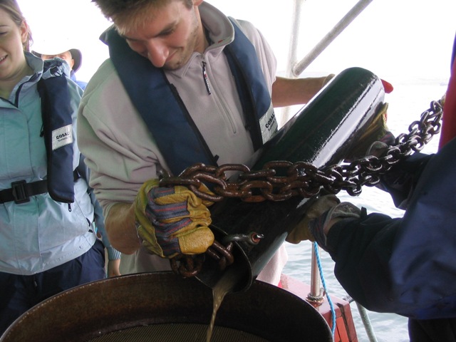
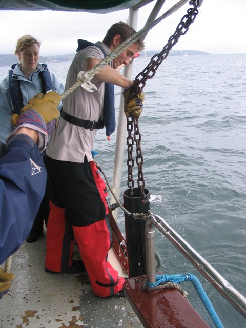
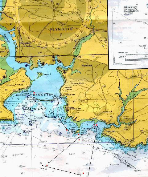
To obtain a representative view of the sea floor, several areas of Plymouth Sound and the River Tamar were sampled using side scan sonar. We surveyed Cawsand Bay, the Breakwater, and the River Tamar. A number of side scan sonar transects, grab samples and pipe dredges were carried out.
Figure 3 shows the track taken while surveying with the side scan sonar. This consists of a survey grid in the area of Cawsand bay to the West, a West to East transect which follows the line of the Breakwater and survey lines up the estuary.
Figure 3 - Survey Track
| Vessel: Natwest II | Departure time: 08:00 GMT | Weather Conditions: | Tide Times: |
|
Poor visibility - low cloud, 8/8ths cloud cover. |
LW 7:20GMT - 1.93m | ||
|
AM showers turning to persistent rain PM. |
HW 13.40GMT - 4.53m | ||
|
Sea state moderate to rough with considerable swell. |
LW 19.50GMT - 1.95m |
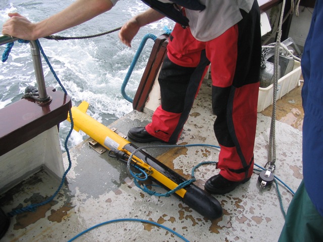
Side Scan Sonar.
Site A - Cawsand Bay
On our arrival at Cawsand Bay, the tide was in a state of flood, here we carried out the following sampling methods:
Side Scan trace :
Start Time: 09:27:14 GMT Finish Time: 10:25 GMT
Start Position: 50° 19.5 N 004° 11.003 W Finish Position: 50° 19.4 N 004° 11.001 W
During one of the transects a distinct change in reflectance from the sea bed was observed on the side scan trace. This area was marked and the positions were noted down. As this was of interest it was planned that two pipe dredges were to be taken either side of the boundary to determine why there was such a change in the reflectance.
|
|
Pipe Dredge 1 |
Pipe Dredge 2 |
Pipe Dredge 3 |
|
Time (GMT) + 1hr BST |
10:45:08 |
11:00:48 |
11:05:48 |
|
Location – Latitude |
50° 20. 001’N |
50° 20. 002’N |
50° 20.003’N |
|
Longitude |
004° 10. 006’W |
004° 10. 006’W |
004° 10. 006’W |
Due to the second pipe dredge failing to collect a significant sample volume, a third pipe dredge was used which consequently produced a good sample.
Site B - Plymouth Sound Breakwater and The Bridge
Due to the Breakwater being a man-made sea defence, surveying the area was of interest in terms of sediment dynamics. The side scan sonar was towed parallel to the breakwater along the northern, inshore side from west to east at around 30 m distance. Figures 4 and 5 show a section of this scan.
Start Time: 11.23 GMT End Time: 11.39 GMT
Start Position: 50º 20.002'N 004º 09.004'W End Position: 50º 20.003’N 004º 08.005'W
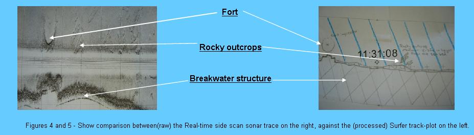
From the two diagrams it can be seen that there is a clear correlation between the side scan data and the surfer plot. The breakwater structure can be seen by the dark undulating line found on the side scan sonar plot. This is replicated on the surfer plot by the crossed hatched section of the diagram.
Site C - Hamoaze and River Tamar
A third side scan sonar transect was undertaken up the main Hamoaze Channel and the Tamar River. Having identified a possible sediment boundary in the confluence of the Tamar and Lynher rivers, three grabs downstream and two further upstream of the Tamar Bridge for comparison were completed.
Start Time: 12.47 GMT End Time: 13.28 GMT
Start Position: 50º 24.005'N 004º 12.002'W End Position: 50º 23.005'N 004º 13.009'W
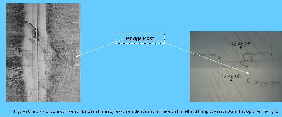
As the above figures show, the rock outcrop which can be clearly seen on the side scan trace to the right as the raised sections which correspond to the drawn area on the track-plot. The same applies to the bridge posts which give a similar, if smaller, reflection to the fort above.
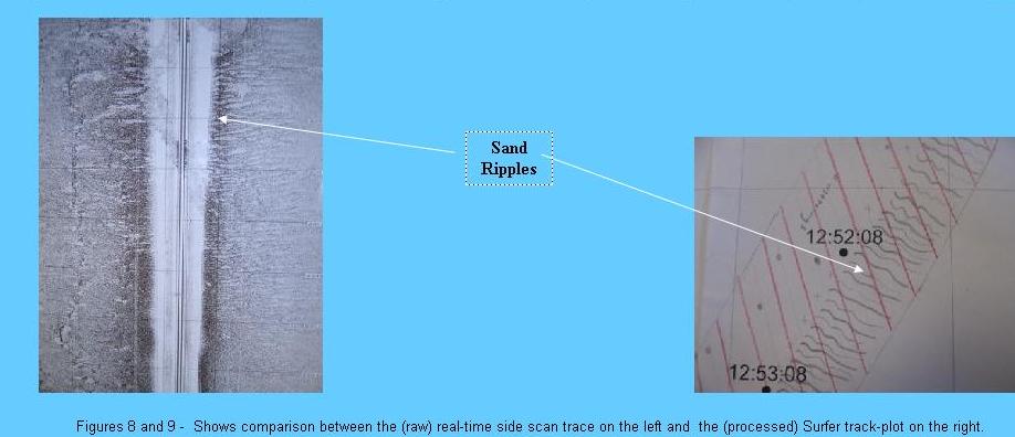
The large sand ripples seen in the track plot (figure 9) and the corresponding side scan sonar trace above are caused by increased current velocities as a result of the narrowing of the estuary below the Tamar Bridge.
Cawsand Bay Pipe Dredge.
The side scan results for the Cawsand Bay area indicated a boundary on the sea bed, suggesting a change in sediment composition. We decided to take a series of pipe dredges to further investigate this. Dredge 1 was taken at 50˚20.1N 004˚10.6W, approximately 100 metres below the boundary line, as shown on the chart. As predicted from the side scan results, the dredge showed a bed of fine sediment and contained many shell fragments and benthic, infaunal organisms such as bivalves. The second dredge was taken above the boundary line, where we expected to see a transgression into coarser sediment. This dredge failed to collect any sediment and a second attempt was carried out in the same area, ensuring that the dredge was at the seafloor and was towed for a prolonged period of time. Dredge sample 3 was taken at 50°20.003'N 004°10.006'W and was found to contain minerogenic material such as shell fragments and showed a general increase in the coarseness of the sediment compared to site 1. The difference in grain size between the two dredge sites supports the presence of a sediment boundary as was indicated by the side scan sonar trace.
Lobster Pots
|
At 10:13:30 GMT a collection of side-scan sonar readings along a sediment boundary were identified. They appear as short dark lines on the finer silt sediment, but with no elevation or depression, running in a south west direction, the same direction as the prevailing winds. There was confusion over what these were but an explanation may have been found. |
 |
The survey area in question is used for lobster fishing, and as such lobster pots are deployed on lines and buoys. As the boat retrieves and reels in the pots the prevailing winds gently push both boat and pots in the southwest direction. This causes the pots to be dragged along the bottom, scraping the overlying silt off the coarse sand. This left just dark tracks of the underlying sediment without producing deep furrows, explaining the size, shape, direction and distance apart. Whether or not this is the true reason maybe up for debate. |
Figure 10 - Shows possible Lobster Pot Scours in Sea bed which cross beneath the path of the survey.
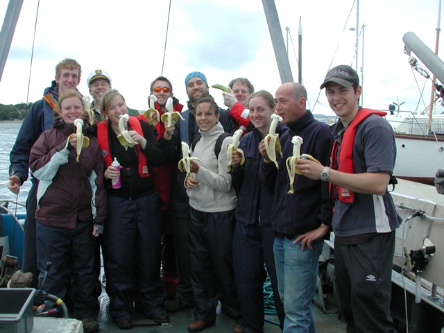
Group Photos from Natwest II

04/05/05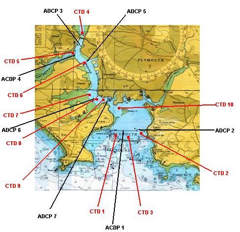
We aimed to investigate the physical features vertically in the water column and spatially along the estuary between the Tamar Bridge and the Breakwater. During our study we were on a neap tide, ebbing for Breakwater sampling, otherwise flooding. To determine the vertical structure with regards to temperature and salinity, a CTD profiler was dropped at eleven sites along the estuary. Ten ADCP transects were also carried out to investigate the direction and speed of water flows. Our sites were chosen to correspond with local influences such as the confluence of two rivers, sewage outfall or observed currents such as around the breakwater. With respect to the physical structure, we expect a more stratified water column further up the estuary where tidal influence is less, and well-mixed water down towards the breakwater. We have chosen 4 sites to demonstrate our findings with respect to an overall physical structure of the estuary. At each site discrete water samples were taken at specific depths, from which the chemical and biological properties of the water will be analysed with respect to nutrients, oxygen and plankton concentrations. They are presented here in geographical order, progressing from the head of the estuary toward the mouth and into Plymouth Sound. For locations, see Figure 11.
Figure 11 - CTD and ADCP transects
Locations – (1) Above the Tamar Bridge
(2) Mouth of the River Lynher
(3) Main channel, near Torpoint
(4) Breakwater
| Vessel: Bill Conway | Departure Time: 08:30 GMT | Weather Conditions: | Tide Times: |
| Fairly calm, small wind waves < 30cm. Swell |
LW 10.10 GMT 1.78m |
||
| Sunny with rain intervals |
HW 16.20 GMT 4.67m |
||
|
5/8 cloud cover |
Physical Analysis – CTD and ADCP data
Location (1) Above the Tamar Bridge
ADCP transect 2 [T2], CTD site 4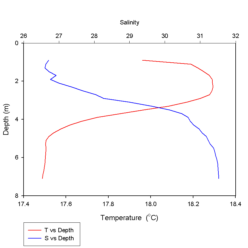
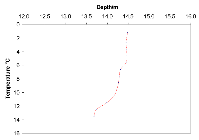
T2 was taken upstream of the Tamar Bridge from West to East bank. The ADCP shows a change in water direction between the upper riverine flow and the landward salt water flow at a depth of approx. 2 metres. As the tide progresses up the estuary, energy is lost due to friction and less energy is available in these higher reaches for mixing saline water across the saltwater-freshwater interface. The system therefore remains fairly stratified.
Application of the Brunt-Vaisala equation to the CTD data at this site gives a frequency of 0.19 radians sec-1 and a period of 31 seconds. A very short period such as this indicates a stable stratified system in which water that is moved from its position of neutral buoyancy is quickly restored to its place. The stratification of the system indicated by the Brunt-Vaisala frequency is confirmed by the CTD analysis, as shown in Figure 12, where the thermocline and halocline are well defined.
Figure 12 - CTD profile for location 1
Location (2) River Lynher ADCP Transect Three [T3], CTD site 6
The T3 transect, shown in Figure 13, was taken across the mouth of the river Lyhner from East bank to West bank. Due to slack water at the turn of the tide, the ADCP shows relatively low water velocities.
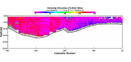 |
The left hand side of the above transect shows that the water body is almost stationary at the bottom due to the pivoting of the water around the corner point, causing a still water profile. This shows us that the water column is well mixed, as we found further up the estuary above the Tamar Bridge. This is further demonstrated by the CTD profile. As the two water masses meet in the confluence of the rivers Lynher and Tamar, turbulence develops creating mixing in the water column causing only a slight and gradual change in both temperature and salinity with depth as shown in Figure 14. This shows that the stratification is less than higher up the river where the two layer system dominates the physical profile but less well mixed than at the tidally mixed waters near the breakwater. |
 |
Figure 13 - Velocity direction from transect 3 Figure 14 - CTD profile for location 2
(3) Main Channel, Torpoint ADCP
Transect Six [T6], CTD sites 7 and 8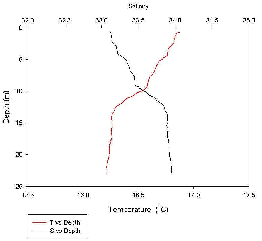
CTD sites 7 and 8 are situated further down the estuary on either side of the main channel near Torpoint. Figure 15 shows the expected fairly stratified system at Station 7 on the West side, as observed further up the estuary near the Tamar Bridge.
Figure 15 - CTD profile for location 3, West Side
 |
On the eastern side of the channel, we identified a possible eddy by the change in water state, Figure 18 shows the surface appearance of this eddy. The turbulence created by the currents associated with the eddy had mixed up the water column, resulting in the much more uniform profile observed in Figure 17. The ADCP profile in Figure 16 gives a visual representation of the eddy current, showing strong currents and the change in water direction through 360o from start to finish. |
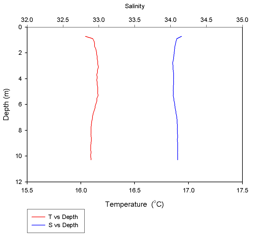 |
Figure 16 - Velocity Direction from transect 6 Figure 17 - CTD profile for location 3, East Side
(4) Breakwater ADCP
transect T1, CTD sites 1,2 and 3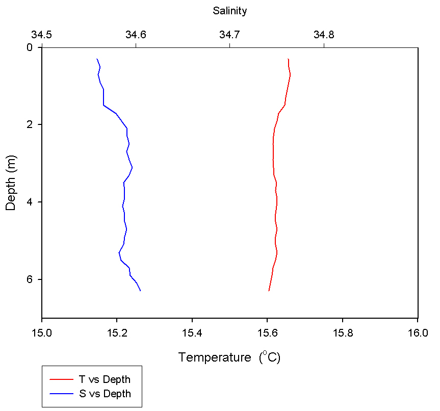
Our most seaward site was at the breakwater, for which we expected the most well mixed water column. The ADCP transect was taken across the inshore side, from the west to the East and shows a change in direction of the water flow of approx. 90o between the two layers; those being the riverine top layer flowing in the seaward direction and the seawater inflow at a depth of 3-3.5meters.
Applying the Richardson equation gives a value of 0.093. This indicates that the internal waves created by the two water masses travelling in different directions will eventually become unstable and break, mixing the water column. At the breakwater, tidal influences are high and breaking waves and passing traffic all create turbulent conditions and further mix up the water column. This is confirmed by the CTD analysis. CTD sites 1, 2 and 3 are all situated around the breakwater and show almost uniform depth profiles for temperature and salinity as shown in Figure 19. Figure 19 - CTD profile for location 4
The chemical and biological features of the water samples taken at each depth can be analysed and interrelated to the physical structure. The data that was collected was combined with another groups RIBs data for the same day to enable a more spatially complete picture to be made. The data we collected on the RIBs was then given to the Bill Conway group for the corresponding day. From this, the theoretical dilution lines for nitrate, phosphate, silicate and oxygen can be constructed for the whole estuary.
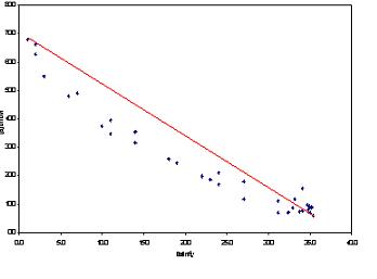
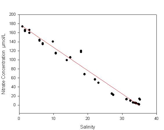
Using the flow injection method, the nitrate concentrations were determined. In general, very high levels of nitrate were found with a maximum of 173 µmol/L at a salinity of 0.93, probably due to heavy rainfall in recent days, increased run-off and nutrient leaching. The theoretical dilution line shown below in Figure 20 indicates that in the Tamar Estuary, nitrate behaves relatively conservatively, although there is slight removal below the theoretical dilution line, possibly due to removal by phytoplankton. The positive outliers in Drakes Channel at a salinity of 35 and further upstream at salinities of approximately 18 and 10 show additional processes, maybe due to increased run-off from local industry.
Figure 19 - Nitrate Mixing Diagram
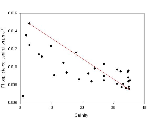
The phosphate concentration of our samples and those collected on the RIBs was determined by spectrophotometer analysis, as shown in Figure 21. The data indicates that as salinity increases, ie; moving down the estuary, phosphate was being removed from the water column, probably taken up by phytoplankton. The most rapid loss of phosphate from the system occurs in brackish water with salinities of between 5 and 18 where phytoplankton concentrations are highest. An increase in concentration occurs from a salinity of 18 at 0.85 µmol/l to a salinity of 27 at 0.12 µmol/l. This shows an input of phosphate in the mid reaches of the estuary, this could be due to input from a sewage outfall in the locality.
Figure 21 - Phosphate Mixing Diagram
The absorbance values for a range of standards were used to obtain the silicate concentrations for the collected samples. In the Tamar estuary, Silicon (Si) behaves non-conservatively i.e. there is removal occurring between salinities 0-34, see Figure 22. This removal is fairly constant between salinities 1- 30. A likely cause would be the uptake of Si by diatoms, which incorporate Si into their cell wall. At salinities of 31-35 there is an increase in silicate. At corresponding salinities the Cattewater enters Plymouth Sound; this may be introducing high levels of dissolved Silicate.When nutrients in estuaries are seen to behave non-conservatively it is often attributed to biological production and degradation processes. (Morris et al., 1981).
Figure 22 - Silicon Mixing Diagram
Phytoplankton, Zooplankton and Oxygen Content
 The
sites of our water samples were decided with the aim of investigating
the implications of the different physical structures discovered in the
estuary. To demonstrate our findings we chose 4 sites to analyse the
change in biological and chemical properties with the change in physical
structure. This includes a stratified system, as found near the Tamar
Bridge
(see Figure 23 ), a frontal
system that we passed in the river Lynher and either side of the
breakwater. We expected to find higher phytoplankton concentrations and
lower oxygen levels in more stratified systems, where we have already
discovered that nutrient levels are high.
The
sites of our water samples were decided with the aim of investigating
the implications of the different physical structures discovered in the
estuary. To demonstrate our findings we chose 4 sites to analyse the
change in biological and chemical properties with the change in physical
structure. This includes a stratified system, as found near the Tamar
Bridge
(see Figure 23 ), a frontal
system that we passed in the river Lynher and either side of the
breakwater. We expected to find higher phytoplankton concentrations and
lower oxygen levels in more stratified systems, where we have already
discovered that nutrient levels are high.
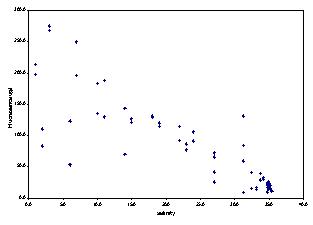
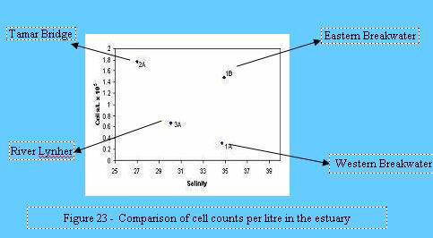
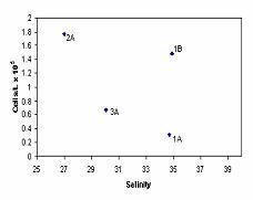
Phytoplankton in the water samples were identified to species level and expressed as cells per litre. Only diatom species were identified in the samples collected. Near the Tamar Bridge, at the lowest salinity, phytoplankton cell numbers were 1765000 cells/L. This corresponds to the high nutrient concentrations in lower salinities as shown in the theoretical dilution lines in Figures 21, 22, and 23. The decrease in cells/L seen from stations 2A - Tamar Bridge to 1A - West Breakwater is supported by the decrease in fluorescence seen between these salinities. Shown in Figure 24.
Figure 24 - Flourescence against salinity for estuarine samples
The high phytoplankton concentration observed, corresponds to a high zooplankton concentration. This was analysed with the use of a zooplankton net trawl.
Zooplankton Trawl Site 2A – North of Tamar Bridge
Haul Surface tow
Total zooplankton; 11750/m³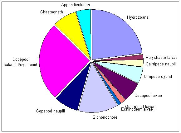
The sample from site 2A shows a high proportion of meroplankton larvae in the zooplankton population, 11750/m3, further up the estuary. See Figure 25. The same can be seen in the when moving from inshore to offshore (see offshore zooplankton analysis). A suggestion for this pattern of distribution is that most larval zooplankton are benthic organisms, therefore in shallower waters there is a smaller water column through which the organisms may disperse. This increases the chance of finding the zooplankton larvae.
Figure 25 - Mesozooplankton counts for the Tamar estuary, site 2A
Combining the
RIBs data from further up the estuary,
it is clear that calanoid and cycloploid copepods make up over 90%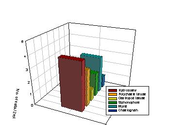 of the entire zooplankton population. The remaining organisms are more clearly
represented in
Figure 26.
of the entire zooplankton population. The remaining organisms are more clearly
represented in
Figure 26.
The next most productive site was the sheltered Eastern Breakwater, site 1B. This corresponds with the high fluorescence values found there, see Figure 24. As in the Tamar Bridge site, the high level of primary production found in site 1B also results in correspondingly high concentrations of the primary consumers, zooplankton, 38000/m3.
Figure 26 - Zooplankton population, excluding calanoid and cycloploid copepods
Zooplankton Trawl Site 1B . East of the breakwater
Haul Surface tow
Total Zooplankton Counts; 38000/m³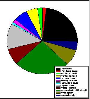
As seen in Figure 27 the dominant species within this sample was again Hydrozoans and Copepods of both the calanoid and cyclopoid genera. It is also notable that there was a wide variety of species within the trawl sample which suggests the water at this position supports a healthy population of phytoplankton that is capable of feeding a diverse community of primary consumers.
Figure 27 - Mesozooplankton counts for the Tamar estuary, site 1B
|
Figure 28 illustrates
the oxygen content in the water varies significantly through the
salinity range. Although there is no distinct correlation in terms of an
increase or decrease with salinity, the amount of oxygen can be linked
to the level of primary producers and consumers in the water at each of
our sites. The high concentration of zooplankton in the East breakwater
and near the Tamar Bridge corresponds with the low oxygen levels also
found there, see Figure 29.
|
 |
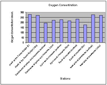 |
Figure 28 - Oxygen concentration vs salinity for the Tamar estuary Figure 29 - Oxygen concentration for each site

In comparison to the East Breakwater, the West Breakwater station (1A), had the lowest number of cells per litre. As discussed previously with respect to the ADCP profile, this area has high levels of disturbance from passing traffic which mixes the water column. Increased mixing may move immobile phytoplankton cells below the euphotic zone or critical depth of the cells, where no net photosynthesis can occur. Mixing through the water column will also decrease the number of cells at any one depth sampled, which may account for the low levels, as observed in Figure 23. The high oxygen concentration in the West Breakwater, as seen in Figure 29, is indicative of the lower levels of primary consumers. This follows as a result of lower levels of primary producers, demonstrated by low levels of fluorescence seen in Figure 24.
In the River Lynher we identified a front by a change in water colour from dark blue to a cloudy green. As we had already established that there are elevated nutrient levels at these middle salinities and with the knowledge that the frontal system may mix up the water column and distribute these nutrients, it was expected that there would be high phytoplankton cell numbers. In fact cell numbers were lower than at station 2A (the Tamar bridge), Figure 23. The fluorescence graph shows low values for the corresponding salinity indicating low chlorophyll and hence supporting the low phytoplankton cell numbers recorded, see Figure 24 This unexpected result may have occurred due to drifting during deployment of the CTD rosette and the collection of the sample from one side of the front.
As an overview of our Bill Conway practical, our CTD, ADCP and water analysis successfully provided us with a spatial and vertical physical profile and allowed us to inter-relate the chemical and biological properties of the water. More specifically, we established that further up the estuary, the water column is stratified because of decreased tidal influence and less mixing across the freshwater-saltwater boundary. There are also high levels of nutrients in these higher reaches due to run-off from the surrounding land. These nutrient levels decrease with salinity down the estuary. Nitrate behaves relatively conservatively whereas silicate and phosphate are significantly removed by phytoplankton. The highest levels of primary production were found near the Tamar Bridge where this stratified structure was most evident. The second most productive area was in the East side of the breakwater where it is sheltered; this, in comparison to the Western Breakwater where traffic disturbs the water column mixing the phytoplankton to below the euphotic depth regularly which means that the phytoplankton populations cannot proliferate, even though they may not be light or nutrient limited before perturbation. The oxygen profiles for these three sites indicate the amount of predation on the phytoplankton by zooplankton, which has given rise to low levels on the East side of the Breakwater and high levels on the Western end of the Breakwater where there are few phytoplankton to predate on, similar high levels are seen in the Tamar Bridge site.
Group Picture from Bill Conway
The aim was to investigate the changing physical conditions when moving from offshore to inshore. We expect to find a more stable and stratified system further offshore, which gets increasingly mixed and homogenous with respect to nutrients and oxygen moving inshore. Because of the shallowing of the sea bed towards the shore, we also expect the mixing lower layers to shift the thermocline further up in the water column. We sampled several sites but selected three main ones to demonstrate our findings. Locations of sampled sites can be seen on Figure 30 .These were:
Station 1 – East Breakwater
Station 5 - Offshore
Station 7 – Inshore, Wembury Bay
Figure 30 - ADCP transects and CTD sites
CTD (See
Figure 31) and ADCP profilers were used to
measure the physical parameters and a plankton trawl and a rosette wate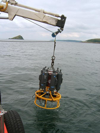 r samples
were taken to investigate the chemical and biological properties. The net used
was 54cm in diameter and could be closed at any depth to retain only plankton
found at specific depth intervals.
r samples
were taken to investigate the chemical and biological properties. The net used
was 54cm in diameter and could be closed at any depth to retain only plankton
found at specific depth intervals.
Station 1 – Inshore, East Breakwater 50o 20.186N 004o 09.423W
Position - Inside the breakwater, west side
Depth - 15.5m
Time - 0835GMT
Weather - 6/8 cloud cover, low winds Figure 31 - CTD Instrument
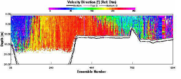
As seen in Figure 33 the ADCP transect shows a change in the flow velocity around the Eastern and Western ends of the breakwater. The blue colour indicates slow moving water behind the breakwater and the fast moving water is represented by the green/red colour. This obvious velocity change occurs as the water trying to leave the estuary must travel around the breakwater, causing the water to move at a greater velocity as it must exit though a narrower gap. This is mirrored in the water movement through the narrows higher up in the river Tamar.
Figure. 32 - CTD Profile for Station 1 Offshore.
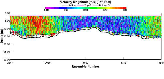
Figure. 33 - ADCP Profile of Station 1 Showing Breakwater.
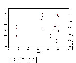
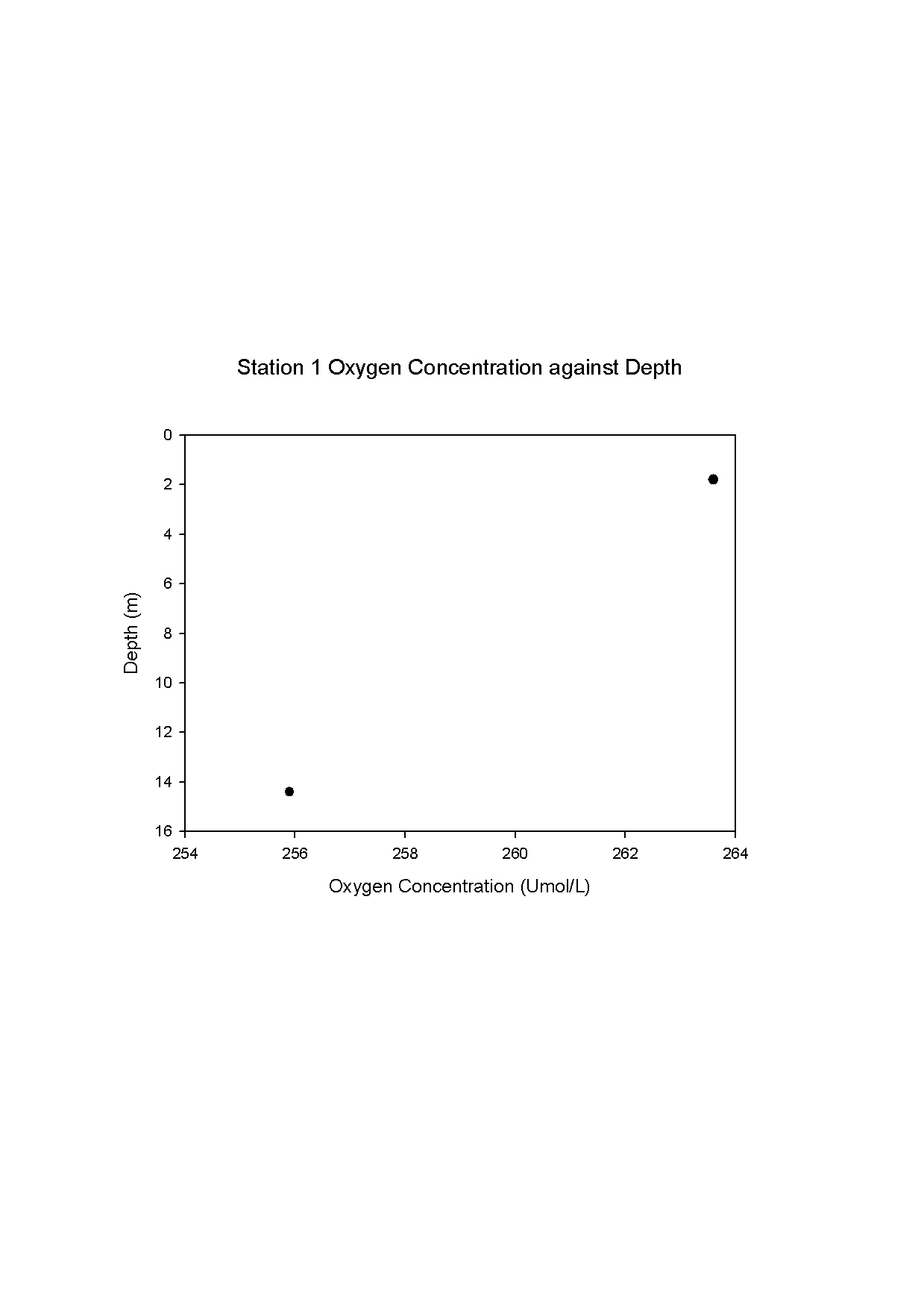
Because of the turbulence created by the fast moving currents and the shipping channel nearby, the water column is well-mixed, as discovered in the Bill Conway Estuarine practical. The CTD profile for the east breakwater, Figure 32 , gives further evidence of the mixed water column with a change of just 1oC over 14m. Because of the mixing, oxygen concentration levels are fairly similar throughout the water column, Figure 35.
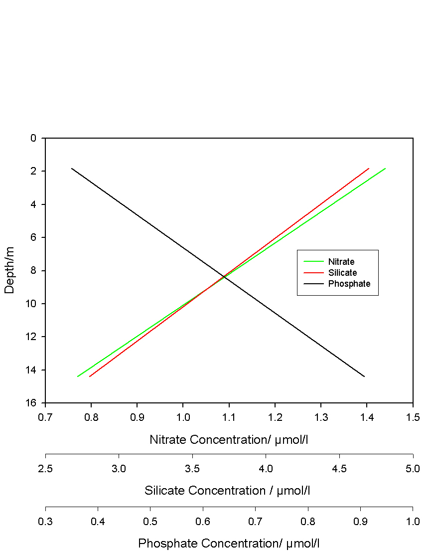
To demonstrate the mixing, two depths were sampled and it was found that nitrate and silicate were at very slightly higher concentrations, 1.45umol/L & 4.54umol/L respectively, in the surface water than at depth. This can be seen in figure 34. However, phosphate concentration was found to be lower at the surface, just 0.34umol/L, than at depth, 0.93umol/L. We would expect nutrients to be depleted in the surface waters following the spring bloom, but the water is well mixed here and the differences in surface and depth concentrations are small and probably just due to small-scale variation in the water column.
Figure. 34 - Nutrients from Station 1 Offshore.
As previously found in the Estuarine practical, there are high levels of primary production throughout the water column in the sheltered Eastern Breakwater area. This is because the Breakwater receives high levels of nutrients from both the riverine and estuarine inputs, more so than offshore areas. A measured Secchi disc depth of 6.3m at this site estimates the euphotic zone to extend to approximately 19m. With a depth of only 15m at this site, this means that primary production can occur throughout the water column.
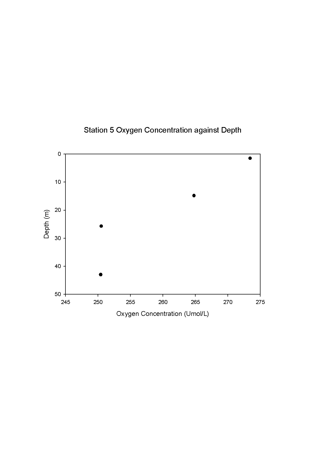
Station 5 – Offshore 50o 15.814N 004o 05.212W
Depth - 45.6m
 Time - 1121GMT
Weather - 6/8 cloud cover, low winds, some sunny spells
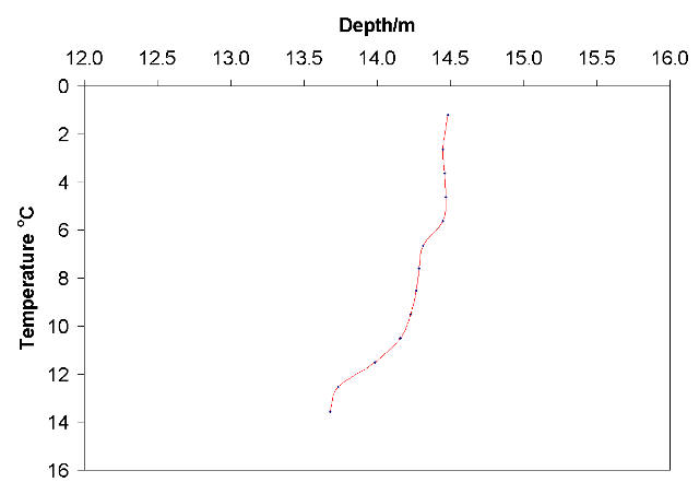
Station 5 was the deepest and furthest offshore station. The water column here was more stratified as expected and the temperature profile clearly shows the two water masses, Figure 36. The seasonal thermocline creates a physical barrier on the ocean this separates the mixed surface layer from deeper waters. It plays an important role as it prevents the transfer of physical and biological properties such as heat, nutrients and algal cells (Sharples et al., 2001).
Figure 35 - Oxygen profile of station 1
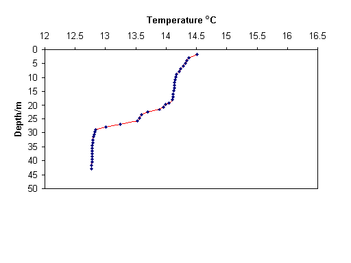
Figure. 36 - CTD Station 5 Offshore
Four depths were sampled and they show that the phosphate is higher in the surface, 1.31umol/L, and depleted at depth, 1.11umol/L, whereas the silicate and the nitrate are depleted at the surface, 0.05umol/L & 1.00umol/L respectively, as we would expect due to phytoplankton uptake. The deeper the water is, the more stratified the water column will be with respect to oxygen, as less mixing occurs in the deeper layers. Figure 36 shows this stratification in comparison to station 1.
A Secchi depth of 8.4m in our most offshore site, estimates a euphotic zone of approximately 25m. While this may be 6m deeper than for station 1, the phytoplankton concentration is lower than for the Eastern Breakwater, because of lower nutrient levels, compare figure 38 to figure 34. Below the euphotic layer where light levels are limited primary production decreases and therefore oxygen concentrations will be lower. Other benthic feeders like zooplankton larvae also lead to these low oxygen levels, see Figure 37. Phytoplankton require a sufficient supply of light and nutrients for net photosynthesis to occur. Therefore, growth within the subsurface maximum requires the thermocline to be situated above the compensation depth along with an upwelling of nutrients from below (Sharples et al., 2001).
Biological activity is also a dominant role to determine the oxygen content of the oceans. It has been found from the water samples that there was a high level of phytoplankton found in the surface layers where sunlight intensity is highest. A Secchi depth of 8.4m estimates a euphotic zone of approximately 25m. Below the euphotic layer where light levels are limited primary production decreases and therefore oxygen concentrations are found to be lower. Other benthic feeders like zooplankton larvae also lead to these low oxygen levels.
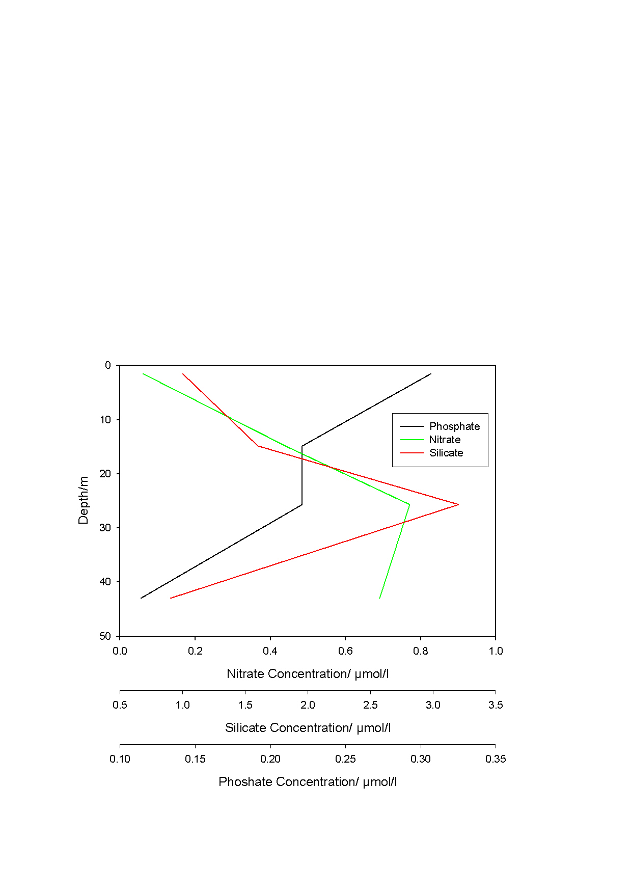
Figure 37 - Oxygen profile of station 5
Figure. 38 - Nutrient Concentration Station 5
 Figure 39 shows an ADCP
transect from the station 5 deep offshore water to the shallower Wembury bay
water. The red colour shows a higher velocity and is localised in a depth of
5-20m, this may be due to tidal flow influence. The boundary between the blue
and green colour is an indicator of two different water velocities running in
different directions. Along this boundary shear and mixing will occur.
Figure 39 shows an ADCP
transect from the station 5 deep offshore water to the shallower Wembury bay
water. The red colour shows a higher velocity and is localised in a depth of
5-20m, this may be due to tidal flow influence. The boundary between the blue
and green colour is an indicator of two different water velocities running in
different directions. Along this boundary shear and mixing will occur.
Figure. 39 - ADCP Transect Five, showing the shallowing of the water
Station 7 - Just outside Wembury Bay 50o 17.499W 004o 05.390W
Depth - 34.8m
Time - 1249GMT
Weather - 5/8 cloud cover, low winds, some sunny spells
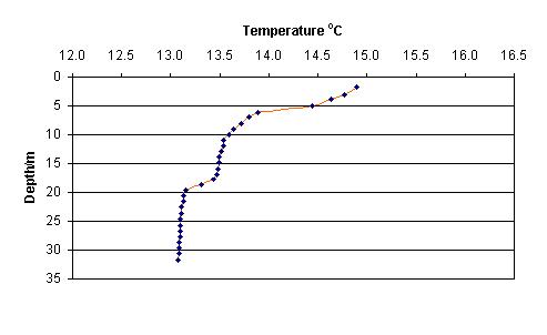
Figure. 40 - CTD from Station 5
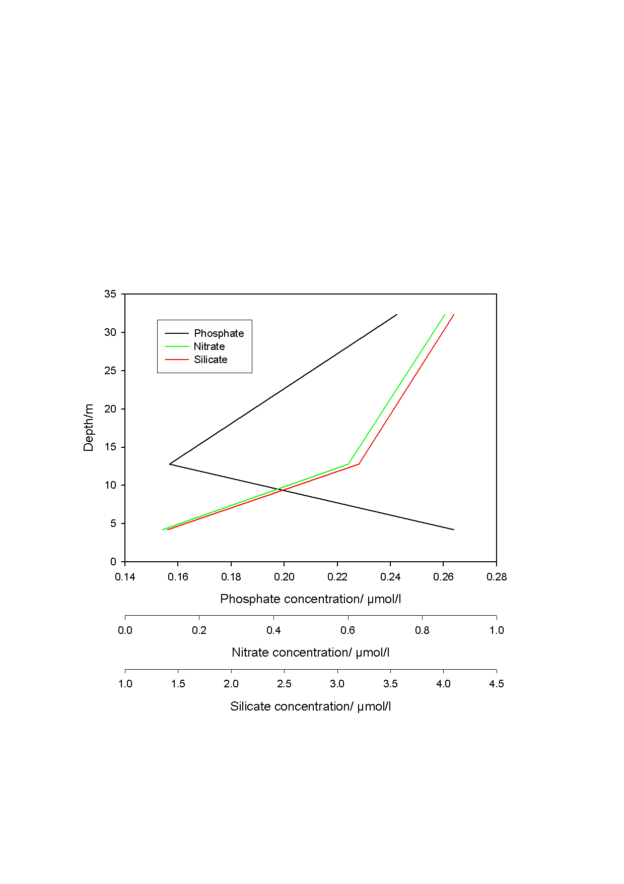
The silicate 1.4umol/L, nitrate 0.1umol/L and phosphate 0.263umol/L concentrations are all higher at the surface and then drop off to the middle depth where the silicate and nitrate continue to fall and the phosphate increases to 0.240umol/L at the deepest sample from 0.158umol/L at 12.5m, see Figure 41. The large concentration of phytoplankton cells found in this area are likely to be situated around this nutricline. Further investigation would help to confirm this.
Figure. 41 - Nutrient Concentration Station 7
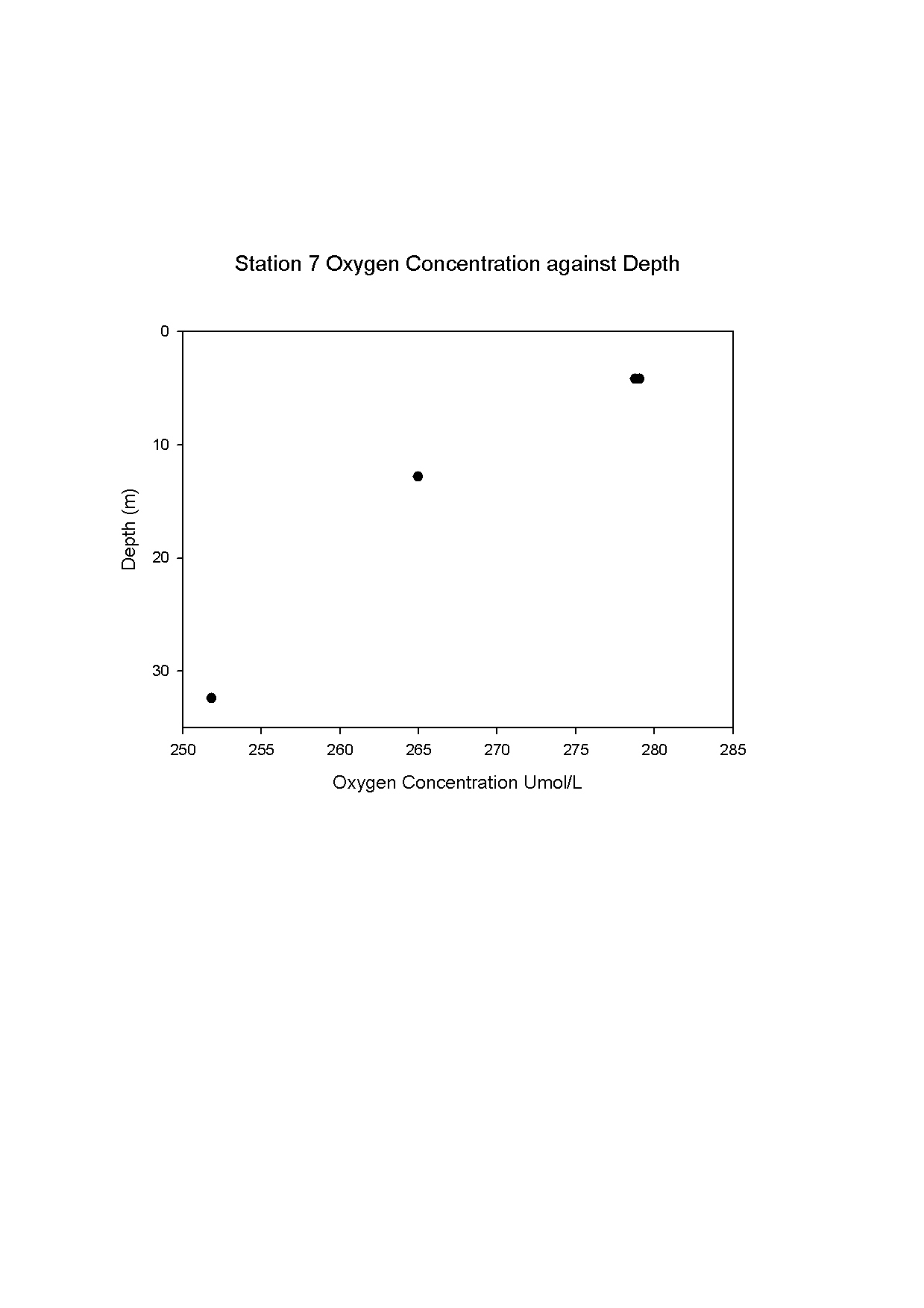
The oxygen concentrations are similar to those of station 1. Oxygen levels are highest near the surface with the lower concentrations found at depth, see Figure 42. As before the highest levels of primary production occurs where light intensity is greatest and decreases with depth.
As the biological content of the water is closely linked to oxygen and nutrient content, we analysed various types of organisms suspended within our samples using a series of net trawls and niskin bottles. Coupled with CTD data it is possible to piece together the chemical, biological and physical processes that drive the waters off the coast of Plymouth
Figure. 42 Oxygen Concentration at Station 7
Analysis of phytoplankton in the waters off of the South West Coast
The South West coast has often been the site of studies (Holligan, 1981) for prominent summer blooms of diatoms and dinoflagellates. The following figures display the various groups of phytoplankton that were collected during the offshore cruise.
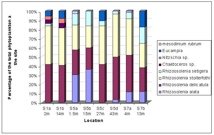
Figure 43 - Proportion of groups of phytoplankton at each sample site
Figure 43 shows that one of the most dominant groups of phytoplankton within the water column at each site is Rhizosolenia stolterforthi, followed by Rhizosolenia delicatula, Rhizosolenia alata and Rhizosolenia setigera which is present in all but 1 site, a sample at 14m depth just inshore of the breakwater.
Both Rhizosolenia dilicatula and Rhizosolenia stolterforthi appear to be prominent at both surface and depth down to 43m. This suggests that these species in particular may be shade adapted (high chlorophyll content) to live at depths of lower light intensities. This would allow the cells to live lower down in the water column below the thermocline where nutrients accumulate having been used up in the surface waters by phytoplankton needing higher light intensities. Rhizosolenia alata and Rhizosolenia stolterforthi appear mainly offshore in the surface waters where numbers of Rhizosolenia stolterforthi and Rhizosolenia delicatula are low and perhaps allow for the growth of other species.
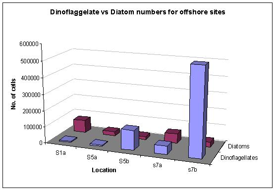
Figure 44 - Proportion of diatoms to dinoflagellates
Whilst analysing samples from zooplankton trawls, it became clear that the net had collected a large amount of dinoflagellates. These accounted for 35% of the total individual zooplankton collected but may have been too large for the phytoplankton filter and thus passed undetected in the phytoplankton samples. Figure 44 shows that the dinoflagellates increase in numbers with increasing distance from the coast and also with increasing depth to 43m. Diatom numbers remain consistent but low relative to the large numbers of dinoflagellates found at site S7b, see Figure 44. Unlike dinoflagellates, diatoms appear in greater numbers closer to the waters surface. This may be because dinoflagellates, being both primary producers and primary consumers can live at low light levels and feed on the phytoplankton from underneath.
Offshore zooplankton analysis, 08/07/04
Coupled with the phytoplankton samples, net trawls were taken at various sites and depths. These samples were then analysed in the laboratory to find and distinguish the different zooplankton species.
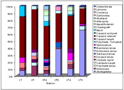
Figure 45 - The proportion of different species within the zooplankton at sites in Plymouth Sound and offshore
The dominant species within the majority of the samples appears to be the Copepod calanoid which makes up nearly 70% of the total zooplankton recorded that day. However, at sites S5B and S7B the dominance of copepod calanoid in the water column is countered by large numbers of dinoflagellates, particularly at site S7B where dinoflagellates make up 65% of the total zooplankton numbers with only 33% Copepods.
From sites 5 and 7 it is evident that there are more dinoflagellates found at depth in the water column than at the surface. This may be because dinoflagellates are both primary producers as well as being primary consumers. Living at depth allows dinoflagellates to utilise the nutrients that accumulate above the thermocline having been consumed and recycled to lower in the water column. Here there is enough light for photosynthesis which means the dinoflagellates have another source of food in the abundance of organic matter, however, at this time of year, there is no shortage of organic matter and dinoflagellate populations can utilise the abundance of light, nutrients and organic matter below the surface water and around the thermocline to grow.
Other species found to be common at each site include siphonophores and hydrozoans although more occur within surface tows.
Zooplankton larvae are proportionally more prominent inshore
RIB’s – 11.07.05
|
Average Weather Conditions: 2/8 cloud cover, very sunny. |
Start Position (Calstock): 50o 29.734N 004o
12.411W Finish Position: 50o 25.657 004o 12.051 |
Start Time: 10:52GMT Finish Time: 13:18 GMT
|
Water samples and temperature/salinity readings were collected along the River Tamar starting from around salinity 3 at Calstock village (site 1) and working downstream. Water samples were collected every 2 salinity change for both chemical (Nitrate, Phosphate, Silicate and Oxygen) and biological (Phytoplankton and zooplankton) analysis. Water Samples were collected towards the Tamar Bridge until reaching 28 salinity. Secchi disk readings were recorded to relate the turbidity to any biological and physical processes occurring at each station.
This Rib data was collected for another research team to compliment their estuarine data from the Tamar Bridge to Plymouth Sound. Figure 46 shows the total survey transect taken. Our upper estuary data was provided by another group for the date 04.07.05 in order to compare the overall physical, chemical and biological processes occurring from River to Offshore. Consequently the data collected in the RIBs on the 11.07.04 is not being analysed by our group for this website.
Figure 46 - Map of Estuarine transect
|
Site |
Longitude |
Latitude |
Temp (ºC) |
Salinity |
Secchi Depth |
Nutrients sample |
Oxygen Sample |
Chlorophyll sample |
Phytoplankton sample |
Zooplankton sample |
|
1 |
50'29.734 |
4'12.411 |
21.85 |
3.11 |
0.21 |
Yes |
|
|
|
|
|
2 |
50'29.734 |
4'12.411 |
20.95 |
4.1 |
0.28 |
Yes |
|
|
|
|
|
3 |
50'29.225 |
4'13.271 |
21.08 |
6.01 |
0.35 |
Yes |
|
|
|
|
|
4 |
50'28.425 |
4'13.254 |
21.31 |
8.13 |
0.37 |
Yes |
|
|
|
|
|
5 |
50'28.380 |
4'13.415 |
20.92 |
10.15 |
|
Yes |
|
Yes |
|
|
|
6 |
50'27.359 |
4'13.672 |
21.97 |
12.22 |
0.57 |
Yes |
|
|
|
|
|
7 |
50'27.338 |
4'13.970 |
21.85 |
14.13 |
|
Yes |
Yes |
Yes |
Yes |
|
|
8 |
50'27.621 |
4'13.511 |
21.52 |
16.32 |
0.63 |
Yes |
|
Yes |
|
|
|
9 |
50'27.706 |
4'13.557 |
21.24 |
10.83 |
0.54 |
Yes |
|
Yes |
|
|
|
10 |
50'27.764 |
4'12.696 |
21.27 |
19.9 |
0.77 |
Yes |
Yes |
Yes |
Yes |
|
|
11 |
50'26.857 |
4'12.373 |
21.08 |
22.45 |
0.96 |
Yes |
|
Yes |
|
|
|
12 |
50'26.656 |
4'12.184 |
20.33 |
25.78 |
0.99 |
Yes |
Yes |
Yes |
Yes |
Yes |
|
13 |
50'25.657 |
4'12.051 |
20.69 |
27.8 |
1.22 |
Yes |
Yes |
Yes |
Yes |
|
Conclusion
The Physical, chemical and biological processes have been studied from the upper reaches of the River Tamar down through the estuary and out into offshore waters. Analysis has allowed us to understand the underlying processes occurring in the estuarine environment. Data has been collected over a two week period by twelve individual groups. This allows a complete data set to be analysed in order to see the periodic fluctuations in the estuary. However it must be kept in mind that empirical field observations can only provide circumstantial evidence of estuarine mechanisms (Morris et al., 1981).
References
Sharples. J., Moore. C.M., Rippeth. T.P., Holligan. P.M., Hydes. D.J., Fisher. N.R and Simpson. J.H – 2001 Phytoplankton Distribution and Survival in the Thermocline. Limnology and Oceanography , 46(3) pp 486 – 496
Tattersall G.R., Elliott, A.J., and Lynn, N.M. 2003. Suspended sediment concentrations in the Tamar estuary. Estuarine, coastal and Shelf Science, 57, 679-688.
Morris, A.W., Bale, A.J. and Howland, J.M. 1981. Nutrient distributions in an estuary;evidence of chemical precipitation of dissolved silicate and phosphate. Estuarine, Coastal and Shelf Science, 12, 205 – 216
Useful links
Group 12 ® - 2005
P.S.Lobster pot man thanks for saving
minibat....man......