Plymouth Field Course 2005
Group 1
![]()
![]()
![]()
Introduction
Over the period of 1st-14th July, the waters off Plymouth, Devon, were sampled with respect to the geological, biological, chemical and physical characteristics unique to the area. In distinct contrast to the sheltered waters of Southampton Water, a group of seven scurvy landlubbers from Southampton University braved the waters surrounding Plymouth and the challenge of gaining a holistic overview of the area's waters.
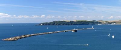
The waters surveyed over the sampling period comprise of Plymouth Sound and the Tamar Estuary. The Tamar estuary is characterised as being a Ria, a drowned river valley. The estuary is 31.7 km in length and is additionally fed into by two tidal sub-estuaries: the Tavy and the Lynher. Its course to the sea flows through the Narrows, a channel of roughly 30m depth, then into and through Plymouth Sound (Tattersall et al., 2003). Mixing within the estuary is varied, with Plymouth sound being relatively well-mixed as a result of its shallow depth and the Tamar Estuary being partially mixed. A 3km wide breakwater was built in the 1800's and is present in the centre of the mouth of the estuary just off Bovisand. It influences mixing processes occurring by protecting the estuary from the strong tidal currents of the Atlantic.
The Tamar Estuary
 OFFSHORE |
|
| Ancillary Data |
Bonito Date: 02/07/05 Time: 0822 - 1420 GMT Weather: wind - SW 8, Visibility - 6, Temperature - 16oC, Sea state - 3/4, Cloud cover - 8/8 Tides: 0210 - 4.5m 0820 - 1.95m 1440 - 4.51m 2050 - 1.93m Neaps |
| Aim |
The aims of this boat practical were to locate the position of the halocline front in the Tamar estuary. The front is the boundary between waters influenced by riverine inflow waters of fully marine characteristics. Changes in the physical properties, such as temperature and salinity, of these two water bodies will identify it's position. These identifiable properties will give rise to chemical and biological activity that will further aid identification of the front's position. |
|
Equipment |
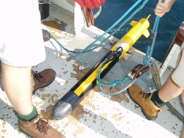
The equipment utilised in the investigation consisted of an ADCP (Acoustic Doppler Current Meter), a CTD profiler, a T/S probe, a plankton net with a mesh of 200µm and a diameter of 0.54m. and a Secchi disc. |
| Method |
The T/S probe was rigged to the hull of the boat, at roughly 15cm. below the surface, this allowed for constant monitoring of the main governing physical properties of sea water during transit. This data was used to identify when the front was crossed and therefore gave an indication as to where samples should be taken. In addition to the T/S probe an ADCP profile was run throughout transit between sampling stations so as to further hint at the front's location. This was achieved through the monitoring of backscatter displayed on the profile which gave indication of rising zooplankton levels, that suggest the presence of phytoplankton, which could be further verified through the application of the Fluorometer and also give indication of the position of the front. CTD profiles were taken to measure the physical properties of the water column. The instrument was situated on a rosette upon which 5 Niskin bottles were attached. Niskin bottles were deployed at depths defined with reference to an ADCP profile of the water column at the station in question. Areas of high backscatter were deemed as being of interest and samples were taken at such depths, other depths of interest included: the thermocline and the surface. The samples achieved through this method were subsequently analysed on return to the laboratory. A vertical plankton trawl was taken from the bottom to the surface of the water column, the net employed was of a mesh of 200 µm and a diameter of 0.54m. Samples were stored in Formalin for laboratory analysis. In addition, a Secchi Disc allowed for the rough interpretation of the depth of the euphotic zone. Samples were taken at: Station1: Breakwater - 50 20.146N 004 09.402W Station 2: Cawsand Bay - 50 19.638N 004 11.141 Station 3: Bovisand - 50 20.073N 004 08.180W |
|---|---|
 Bonito braves the seas
Mark & Jeremy deploy the rosette sampler.
The rosette sampler |
|
|
Results
Figure 1.3 Fluorescence and Transmittance v. Depth for Station 5
Figure 1.6 Fluorescence and Transmittance v. Depth for Station 3
Figure 1.9 Fluorescence and Transmittance v. Depth for Station 4
Figure 1.12 Fluorescence, Temperature and salinity vs. Depth at Station 2
Figure 1.12 Fluorescence, Temperature and salinity vs. Depth at Station 7
Figure 1.13 Nutrient concentrations vs depth at Station 1.
|
Zooplankton
Figure 1.1 Zooplankton distribution at Stations 1,2,3 Numbers of copepods increased from 15% to 42% from station 1 to site 3. Hydrozoans decrease from sites 1 to 3, decreasing from 52% to 6%. In site 2, both hydrozoans and copepods are fairly equal, and in a balance. Most species of zooplankton maintained similar numbers at the three stations tested. The Copepod population increased between stations 1-2 and 2-3 in proportion to the reduction in the hydrozoan population. Since only one net was taken at each station, the only comparisons which can be made are those between stations themselves. In sites 2 and 3 there are no arthropods present. Chaetognaths increase from samples 1 to 3, from 1.4% to 8.3%. This may be due to site 3 being further away from the Tamar estuary, than station 2. Phytoplankton
Figure 1.2 Distribution of Phytoplankton at Stations 1,2,3 Station 1: Two samples were taken at depths of <1m, and 14m down the water column. From this it could be seen that the increase in Nitzschia sp. (as a percentage of the total phytoplankton present in the sample) is equal to the decrease in Rhizosolenia stolterfothii down the water column, with no notable change in the abundance of other species. Station 2: Three samples were taken at depths of <1m, 5.5m, and 12m down the water column. The trend seen at this point was different to that seen at station 1, with an increase and decrease in Chaetoceros sp. (as a percentage of the total phytoplankton present in the sample) being comparable to the sum decrease and increase (respectively) of Rhizosolenia delicatula and Rhizosolenia stolterfothii. Station 3: Both samples were taken at the surface due to equipment difficulties; the values of phytoplankton numbers showed little to no difference between the samples. Physical Properties Station 5: 50 19.638N 004 11.141W 2.5-8.5m Gradient Ri = 0.681 9.8-11.5m Gradient Ri = 2.026 12.8-13.5m Gradient Ri = 0.090 The Richardson Number calculated for offshore Station 5 shows that the water column is stratified down to a depth of around 11m, below which it becomes mixed, although the Richardson number of the first, sub-surface, section is low enough to be indicative of recently mixed water.
Figure 1.4 Velocity magnitude for Station 5
Figure 1.5 Average backscatter for Station 5 There is increased backscatter at surface and at depth, as shown on Figure 1.5. Through comparing this data with the data supplied by the CTD, Figure 1.3, it can be seen that whilst the surface backscatter is indicative of the presence of phytoplankton, shown by high fluorescence, the backscatter at depth does not correlate with this data that shows a drop in fluorescence but an increase in transmittance. Owing to inconclusive data achieved, the data from Group 8 who also sampled with a view to finding the front off Plymouth Sound has been further analysed. Group 8, Station 3: 50 19.077N 004 10.690W 1.5-4.1m Gradient Ri = 0.098 6.0-8.2m Gradient Ri = 0.353 10.1-16.0m Gradient Ri = 129.942 The Richardson numbers indicate that the top water layer is mixed, the central layer is close to mixing and the bottom layer is stratified.
Figure 1.7 Velocity magnitude for Station 3
Figure 1.8 Average backscatter for Station 3 The backscatter profile shows an increase at around 7m depth. The fluorescence and transmittance profiles displayed in Figure 1.6 indicate that this is due to the presence phytoplankton as a result in that a high fluorescence and low transmittance is featured at this depth. Group 8, Station 4: 50 18.378N 004 11.740W 4.9-9.9m Gradient Ri = 0.185 10.4-19.8m Gradient Ri = 1.492 The Richardson numbers from CTD dip 4 shows two main water layers, with the shallower being more likely to mix than the other at depth. The velocity magnitude profile clearly shows two layers moving at different speeds. The deeper, more stratified layer is moving at around 0.15m/s slower than the shallower one.
Figure 1.10 Velocity magnitude for Station 4
Figure 1.11 Average backscatter for Station 4 The backscatter profile shows an increase at around 5-10m depth and again at 17-22m depth. By looking at the fluorescence and the transmittance level displayed in Figure 1.9 it can be seen that this peak points to a high presence of phytoplankton whilst the point at depth shows no peak in fluorescence but a slight increase in transmittance, indicating that it is probably churned up sediment causing the backscatter. Surface temperature is lower at stations further inshore than those offshore by a difference of approximately 0.5˚C. A general trend of decreasing temperature with depth is featured at all stations. The thermocline is pushed to the surface further inshore, at stations 2 to 4 it is featured at roughly 5 metres depth. This decrease in temperature below the thermocline is increasingly pronounced the further offshore the station. Additionally the thermocline appears to deepen with distance offshore. Surface salinities are lower at approximately 34.75 until station 5 is reached, after which it increases to roughly 35.25. With a progression offshore there is a general trend in increasing homogeneity of Salinity down the water column. Station 2 is the closest inshore of all those sampled, at this location salinity is lower at the surface and increases after a depth of approximately 5 metres where a very slight halocline is featured, Figure 1.12. This general trend continues in all stations until Station 5, where salinity increases from the surface to roughly 5 metres after which salinity is constant until 10 metres where it increases rapidly to approximately 35.25. Surface fluorescence is at its maximum inshore at approximately 1.5 Volts, this decreases slightly towards Station 5. At Stations 6 and 7, fluorescence is significantly less at approximately 1 Volt. Stations 2 to 4 feature a maximum in fluorescence at roughly 8 metres depth below which a slight decrease is featured; this decrease is more pronounced with increased distance from the shore. A maximum in fluorescence appears to deepen with distance offshore. Nutrients A primary difference in the relative concentrations can be observed; nitrite and phosphate are in ranges of tenths of a µmol/l whereas silica is in the range of tens of µmol/l. Phosphate and nitrites follow a similar pattern where concentration are elevated at surface depths before slightly decreasing at depths of 5.5m before doubling its relative concentrations to around 0.4 µmol/l. Silica appears to be a small concentration at surface and depth whilst increasing drastically to nearly 20 µmol/l at 5.5m.
Figure 1.14 Percentage Nutrient distribution at Station 1 Figure 1.15 Percentage Nutrient distribution at Station 2
Figure 1.16 Percentage Nutrient distribution at Station 3There appears to be a progression in percentage from site 1 through to site 2, notably the increase in the proportion of silica from 55% to 71% at site 2 and up to 94% at site 3. Consequently the proportion of phosphate and nitrite decrease from nitrite having the dominant proportion between the two nutrients to being equal at 3%. At station 1 (the breakwater), temperature varies significantly with depth, with a decrease from 15.9°C at the surface to 14.4°C at 10m depth. There is an indication of a thermocline at about 5m depth. Nutrient concentrations appear to also decrease with depth. This correlates to an increase in phytoplankton concentrations at the same depth. Table 1.a displays the chemical compositions of the water column at all 3 stations sampled on the 2nd July 2005. With reference to this table it can be observed that there is a general trend of decreasing nutrient concentrations at depth.
Table 1.a Chemical composition of water column at Stations 1,2,3 |
|
Discussion
Figure 1.17 Temperature vs. Depth for Station 1
Figure 1.18 Temperature vs. Depth for Station 2
Figure 1.19 Temperature vs. Depth for Station 3 |
Zooplankton Overall it can be said that the zooplankton analysis was hindered by a lack of stations and therefore data sets. The only pattern appears to be the relationship between the populations of hydrozoans and copepods, which is entirely within reason since hydrozoan zooplankton feed on copepods. Phytoplankton The overall numbers of phytoplankton down the water column fluctuated down the water column, this was probably due to the increased mixing on the day of sampling, with the wind from the southwest at 15knots kicking up a sea state 3-4. The relative percentage composition of the phytoplankton found showed major differences, this was probably due to the relative ease of mixing of different species/groups. Physical Processes With a progression offshore the waters sampled became decreasingly influenced by the freshwater inflow from the Estuary, this is shown by the increasing salinity and a homogenous vertical distribution of this higher salinity featured at Stations 6 and 7. The lower surface salinities featured at the more inshore stations can be attributed to the freshwater influx flowing into the estuary at the surface, this will have been further enhanced both in the data collected by Group 1 and 8 as the weather conditions had been very wet both on and previous to the 2nd and 3rd of July respectively, the days on which sampling took place. The shallowing of the thermocline can be explained by the increased turbulence as the water depth shallows and friction with the sea floor increases turbulence and mixing in the water column. Surface heating is therefore competing against this mixing in such a way that a thermocline cannot be formed before the heat is mixed through the entire water column. Mixing offshore is less pronounced in that the deeper water requires a much larger amount of energy for it to mix over its entire depth. Therefore, the formation of a thermocline is favourable and surface heating results in a more stratified water column further restricting any mixing occurring. This is further supported by the data achieved through the use of the ADCP, with reference to Stations 5 and 8 where an increase in stratification can be observed with distance offshore. Fluorescence is a representation of the level of chlorophyll and therefore a good indication of phytoplankton presence. The deepening of the maximum in fluorescence observed with a progression offshore can be seen to coincide with an increase in the depth of the thermocline. This suggests that the distribution of chlorophyll is governed by mixing as well as a reduction in riverine influence which we can assume to involve suspended matter which affects the euphotic depth. The significant change in both general vertical distribution and surface fluorescence across and either side of Station 5 suggests that the front is situated at approximately this location. This again is supported by the backscatter featured frequently just below the surface which was indicative of the presence of phytoplankton and that near the sea floor which was generally representative of the shear at the water-sea floor interface driving sediment into suspension. Nutrients With a closer look at the nitrite and phosphate concentrations it should be noted that the presence of higher concentrations at the surface depths are indicative of the freshwater input to the estuarine system from surface land run-off. Inputs of phosphates from local sewages plants and industry would ensure a concentration above that of the natural occurring concentrations of trace components. Similarly nitrates reach the water from overflow and badly managed application of fertilizers on crops and surrounding agricultural land which is washed in the river system by higher than average rainfall. Silica should have a uniform input as its concentration is background input from the rocks of the surrounding geology. The weeks previous to the sampling period featured a period of good weather, this may have lead to phytoplankton concentrations increasing in the warm surface waters, utilising all the nutrients. With the rapid decline in nutrient concentrations at the surface, phytoplankton may then migrate to depth to seek more. Prior to this investigation there were three to four days of unfavourable weather conditions featuring a large amount of precipitation. The stronger winds may have lead to increased mixing occurring throughout the estuary, and nutrients, which are in high concentrations below the surface layer, being brought to the surface. At
station 2 ( At station 3, (Bovisand), the thermocline is at a depth of about 4m. Unfortunately due to the problems occurring with the CTD, samples were only taken at the surface at the site. Fluorescence from the CTD data indicates high phytoplankton concentrations at depth rather than at the surface. On comparison with these data collected by Group 8 from a similar site similar trends to that featured to Bovisand can seen. Nutrient concentrations seem to be in the highest quantities at depth of around 10m. This coincides with the chlorophyll maximum, where the large quantities of nutrients in the area allow phytoplankton populations to flourish. However, the station sampled at Bovisand is a much more sheltered environment and so phytoplankton levels are likely to be higher. |
|
Conclusions |
Measurements regarding the physical properties of the water column were,
on this occasion, difficult to obtain. In part this was due to faulty
equipment the problems with which were exacerbated by unfavourable weather
conditions. Owing to such problems these data collected is limited and
unrelated and therefore difficult to analyse and so data from Group 8 who
also sampled with a view to locating the front in the waters just off
Plymouth was further analysed. With regards to the physical analysis of the data collected by Group 1 and 8 an increase in stratification can be seen to occur with a progression offshore, with regards to the front expected just offshore it would appear to have been present at approximately Station 5 sampled by Group 8. This conclusion is drawn with regards to the jump in surface temperature at stations either side of this point and the significant changes in the distribution of nutrients throughout the water column that also occur. The sampling station L4 sometimes represents the tidal front of the region. The location of L4 changes seasonally, in summer it is located between stratified and transitional mixed waters, (Rodriquez et al, 2000). Due to the varying location of the front, we would have had to have taken several more samples around the location of L4 to locate it. |
Introduction
In order to obtain a thorough overview of the processes occurring within the Tamar Estuary, it's entire length was sampled using both the RIBs and Bill Conway. With the Estuary being sampled on two days comparisons can be drawn to aid such conclusions. The work conducted by the RIBs (Rigid Inflatable Boats) was focused on the shallow upper estuary, with the Bill Conway working in the deeper lower estuary.
The Tamar is a tidal estuary where salinity within the main body varies considerably in response to changes in the rate of freshwater runoff and tidal state (Morris et al., 1980). The ebb and flood of the tides has a strong influence on the mixing within the estuary. The mixing of the fresh and saline waters determines the distribution of both the physical and chemical properties of the water. This therefore determines any biological activity that may be occurring. The use of the river's catchment area further influences the chemical activity within the estuary with agricultural and sewage works being of strong influence on the level of Nitrates and Phosphates occurring in the estuary.
|
Calstock |
|
|
Ancillary Data |
RIBs Date: 05/07/05 Time: 0815 - 1710 GMT Weather: wind - S 19, Visibility - 12, Temperature - 15oC, Sea state - 2, Cloud cover - 6/8 Tides: 0444 - 4.7m 1103 - 1.5m 1702 - 5.0m 2327 - 1.4m Neaps |
|
Aim |
To survey the entire length of the estuary with respect to the physical processes and the consequent controls exhibited upon chemical and biological activity within its waters. So as to obtain an overview of the estuary as a whole and it's unique characteristics. |
|
Equipment
Coastal Research
Ocean Adventure |
In order to obtain water samples for laboratory analysis various equipment was needed. The following list contains the equipment used and the reasons for its use.
|
|
Method
Ocean Adventure and Coastal Research
at Calstock |
In order to obtain sampling locations, the CTD was trawled alongside the vessel to allow a constant salinity reading. The group was split into two sub-groups, one operating on each vessel, and readings were taken from zero salinity and then at intervals of three up to a maximum value that was found at 32, with each group sampling every alternative value. Samples were taken for laboratory analysis of Silica, Phosphate, Nitrate, Chlorophyll, Phytoplankton and a net was deployed at one position for the analysis of zooplankton. |
|
Results
Tom and Sian enjoy filtering prepare the samples for analysis
Jeremy and his (T/S) probe
Figure 2.3 Temperature profiles for Stations 1-8
Figure 2.7 Temperature, Fluorescence, Salinity and Transmittance vs. depth at Station 4
Figure 2.11 Temperature, Fluorescence, Salinity and Transmittance vs. depth at Station 7 |
Phytoplankton
Figure 2.1 Phytoplankton distribution at Stations 1-8 Nitrate: Total phytoplankton numbers generally lie between 75000 and 250000 with one seemingly anomalous result at 566850. Diatom population generally lies between 75000 and 250000, but also has one anomalously high result at 560450. Dinoflagellate population ranged from 0 to 89.4 with a 1700 anomaly. Ciliate population showed a random spread pattern. Phosphate: There was also no correlation between phosphate concentration and total phytoplankton numbers. One high result at 0.026µmol dm-3 but otherwise a random pattern lower down. Silicate: There is a distinct lack of silicate values between 17 and 50µmol dm-3 within a spread from 1 to 70 and an anomaly at 566850 µmol dm-3. Diatom population also appears to be randomly spread in comparison to Silicate with one high result. Dinoflagellates show no correlation with silicate concentration. Ciliates show no correlation with silicate concentration. Salinity: Diatom population fluctuates widely as salinity between stations increases, Dinoflagellates spread randomly from populations of 0 to 1700 fro increased salinities. Ciliates have a random spread pattern. Total phytoplankton are spread quite randomly, to see a very weak positive correlation would be optimistic. Zooplankton
Figure 2.2 Zooplankton distribution at Station 3, 6,8 Zooplankton displays a random pattern of distribution. Physical Properties Figure 2.3 shows the temperature profiles produced from the CTD data attained at each site. It is clear to see that there is a significant variation in profiles from the far right plot (Station 1, north of the breakwater) to the far left plot (Station 8, the Tamar Bridge). Temperature progressively become warmer as the investigation progressed up the estuary. Temperature begin at 15ºC at the breakwater, and increase to 17.5º at the Tamar estuary
Station 4: 50 24.642N 004 12.210W
The Richardson numbers for this CTD site show two fairly stratified layers of water. The slight difference can be seen on the velocity magnitude profile, and two different speeds are shown on the velocity direction profile. The differing speeds and directions may indicate a possibility of mixing as the shear will be higher than it would with two similar moving layers travelling in the same direction. This friction would cause turbulence and so mixing would probably occur.
Figure 2.4 Velocity Direction for Station 4
Figure 2.5 Velocity Magnitude for Station 4
Figure 2.6 Average backscatter for Station 4
The decrease in fluorescence and slight increase in transmittance with depth indicates that the peak in backscatter at depth is most likely due to churned up sediment featured in Figure 2.7. Station 7: 50 21.975N 004 11.452W 0.9-8.5m Gradient Ri = 0.336 9.1-13.9m Gradient Ri = 1.768 The second Richardson number shows a fairly stratified layer of water, the first number indicates a body more likely to mix. The velocity magnitude profile shows that the two layers are travelling at a fairly similar speed, though the top layer is slightly faster. The layers are travelling at slightly different directions according to the velocity direction profile. This slight difference in both speed and direction of flow are not indicative of a system that will mix quickly.
Figure 2.8 Velocity direction for Station 7
Figure 2.9 Velocity magnitude for Station 7
Figure 2.10 Average backscatter for Station 7 The high amount of backscatter at the surface is probably due to bubbles produced by the vessel, but the reasonably high backscatter sub surface – between about 2-8m depth are most likely due to the presence of phytoplankton, this is further supported by the increase in fluorescence over this depth, which is displayed in Figure 2.11. The decrease of fluorescence and the increase in transmittance indicate that the backscatter at depth is due to churned up sediment. Nutrients
Figure 2.12 Nutrients and Chlorophyll distribution against Salinity Figure 2.12 shows a decrease in all nutrient concentrations as data was collected progressively down the estuary. Both nitrite and silica decrease fairly continuously down the estuary. Nitrite shows mostly conservative behaviour, deviating from the Theoretical Dilution Line at lower salinities indicating subtraction, this is displayed in Figure 2.13
Figure 2.13 Theoretical dilution line for Nitrite Figure 2.14 Theoretical dilution line for Phosphate Figure 2.15 Theoretical dilution line for Silica Silica displays the general trend of decreasing with a corresponding increase in salinity. The variability in its concentration indicates that it is a non-conservative component of the estuary's waters. From Table 2.a it can be observed that phosphate, nitrate and silica all decrease with depth at all stations sampled in the estuary.
Table 2.a Nutrient Concentrations at all Stations sampled
Figure 2.16 Base of the Euphotic zone calculated via use of a Secchi Disc down the estuary Figure 2.16 shows that the depth of the Euphotic zone increases exponentially with salinity and therefore distance down the estuary. Oxygen The oxygen data collected indicates a slight increase in oxygen concentrations with a progression down the estuary into a more marine environment with a maximum featured at a salinity of approximately 29. After this maximum a slight decrease in concentration is featured at the top salinities sampled: approximately 32 and above. The zooplankton data collected from this area indicated fairly large concentrations, with a total of 70125 organisms collected from a 500ml sample. |
|
Discussion
Figure 2.17 Temperature, Fluorescence, Salinity and Transmittance vs. depth North of Tamar Bridge
Figure 2.18 Temperature, Fluorescence, Salinity and Transmittance vs. depth the Narrows |
Plankton Phytoplankton samples taken at stations throughout the length of the estuary and offshore were identified and quantified by microscopy, after which they were analysed with relation to the in situ salinity and concentrations of nitrates, phosphates, silicates, and oxygen. Previous studies in similar areas (e.g. Sims et al. 2004, Nichols 1998) had led to the expectation that phytoplankton populations would be dependant upon essential nutrient concentrations such as Nitrates, Phosphates and Silica.. This was not supported by the samples gathered in the river Tamar and Plymouth Sound on the 5th July 2005. When analysed it was found that the phytoplankton numbers and composition showed much variation, but no correlation when plotted with the salinity or concentrations of nitrates, phosphates, and silicates. There was also no correlation between the populations of set groups of phytoplankton species (e.g. Diatoms, Dinoflagellates, etc.). Since only three trawls were conducted there is insufficient data to find any correlation between distance down river and the population of varying groups of zooplankton. This said, the population of the zooplankton group and species vary so greatly between stations, it is hard to see how a pattern could arise. Many species of plankton (particularly phytoplankton) look very similar, it is believed that counting errors may have arisen due to mistaking one species/group for another. Using a group of students for the taxonomy may have increased the occurrence of such errors, but other data sources collected in the area over the consecutive few days no correlations either. Physical Processes The sample taken just north of the Breakwater indicates that the water is fairly well mixed, with temperatures remaining fairly constant at 15°C throughout the majority of the water column. Below depth of 8m, both temperature and phytoplankton decrease. As the boat progresses inshore towards the input of the River Plym at Cattewater, temperatures again are fairly constant throughout the water column. There is a steep salinity gradient below the surface water, (1.5m depth), reflecting the mixing of the fresh water input from the River Plym and the saline water of the Sound. Phytoplankton concentrations are at a fairly constant level throughout the water column, with a very slight decrease below depth of 4m. Both silica and phosphate levels decrease fairly rapidly with depth at this site. Silica drops from a concentration of 2.76 µm/l at the surface, to a concentration of 0.78 µm/l at 6m. The freshwater from the River Plym contains high concentrations of nutrients, of terrestrial origin, that are not mixed into the saline water below. This may explain the decrease in phytoplankton concentration below 4m.
Further up the estuary, North of the
Nutrients The sample taken just north of the Breakwater indicates that the water is fairly well mixed, with temperatures remaining fairly constant at 15°C throughout the majority of the water column. Below depth of 8m, both temperature and phytoplankton decrease. As the boat progresses inshore towards the input of the River Plym at Cattewater, temperatures again are fairly constant throughout the water column. There is a steep salinity gradient below the surface water, (1.5m depth), reflecting the mixing of the fresh water input from the River Plym and the saline water of the Sound. Phytoplankton concentrations are at fairly constant level throughout the water column, with a very slight decrease below depth of 4m. Both silica and phosphate levels decrease fairly rapidly with depth at this sight. Silica drops from a concentration of 2.76 µm/l at the surface, to a concentration of 0.78 µm/l at 6m. The freshwater from the River Plym contains high concentrations of nutrients, that are not mixed into the saline water below. This may be the reason for the decrease in phytoplankton concentration below 4m. Further up the estuary, North of the Tamar Bridge, temperature varies quite substantially with depth. At the breakwater there is a slight indication of a thermocline at a depth of 8m, in the Narrows, slightly further up the estuary, there is a strong thermocline at a shallower depth of 4m. North of the Tamar Bridge there is only a slight indication of a thermocline and it is raised to a depth of 2m. The thermocline became much shallower with depth as samples progressed up the estuary. This is due to the water becoming shallower. The decrease in water depth forces the bottom water upwards, leading to mixing. This results is thermocline being much shallower. The fresh surface water has various inputs of nutrients, such as high amounts of phosphates from fertilizers and phosphates and varying other nutrients from the sewage disposals. The nutrients are not mixed throughout the water column and so remain at the surface in higher concentrations. |
|
THE TAMAR ESTUARY: BILL CONWAY |
|
| Ancillary Data |
Bill Conway Date: 12/07/05 Time: 0800 - 1400 GMT Weather: wind - E 5, Visibility - 14, Temperature - 24oC, Sea state - 1, Cloud cover - 2/8 Tides: 0255 - 1.5m 0909 - 4.6m 1504 - 1.7m 2113 - 4.8m Neaps - Springs |
|
Aims
|
To enforce the conclusions drawn from analysis of data collected on the 5th and obtain an informed overview of the Tamar Estuary. |
|
Results
Bill Conway
Figure 3.3 Temperature profiles for all stations
Figure 3.4 Temperature and Salinity vs. depth for station 2
Figure 3.5
Temperature and Salinity vs. depth for station 8
Figure 3.6 Gradient Richardson Numbers vs. Depth at Station 2
Figure 3.7 Gradient Richardson Numbers vs. Depth at Station 8
Figure 3.11 Nutrient and chlorophyll concentrations Vs. salinity |
Phytoplankton The total phytoplankton population increases with an increase in both phosphate and nitrate concentrations and decreasing salinity. The relative abundance of species is dominated by chaetoceros sp. throughout the samples, but other species make up a greater proportion in the lower phosphate/nitrate areas.
Figure 3.1 Phytoplankton distribution up the Estuary, West Mud and the Breakwater Zooplankton Zooplankton population shows no real remarkable change in number or composition between the three stations. It can be seen however that the Cirripedes make up a greater percentage of the total zooplankton population in the river than near the breakwater.
Figure 3.2 Zooplankton distribution up the Estuary, West Mud and the Breakwater Physical Properties A general increase in temperature is seen as one progresses along the estuary from the breakwater to the Tamar Bridge from 16 degrees to 20.5 degrees. The water flowing down the river Lynher sampled at the mouth, site 7, is significantly cooler than the water body sampled at site 6, St. John’s Lake. St. John’s an area which is exposed at low tide. At the time of sampling the tide had been ebbing for about an hour and a half and so the water out flow was relatively higher than the water flowing out of the mouth of the Lynher. When plotted on a T/S profile the two extreme stations at the ends of our sampling area show an inverse relationship of temperature against salinity. At st 2, again we see an inverse relationship of Temperature against Salinity, with warmer river water affecting the thermocline and the presence of different water bodies. This is reflected by the slight changes in salinity at depths of around 6.8 and 12m (Fig 3.4). The temperature at these depths is inversely proportional to these changes in salinity. Figure 3.6 shows the variation in Gradient Richardson numbers (Ri numbers) down the water column at the site of the 6th CTD drop, 50 23.371 N 004 11.953. NB The numbers are plotted on a logarithmic scale in order to accommodate the Ri numbers that reached infinite proportions. These infinite Ri numbers are plotted on the graph as 500.
Figure 3.8 Velocity Magnitude for Station 2
Figure 3.9 Velocity Direction for Station 2 Figure 3.8 shows that the water is stratified from the surface down to a depth of just below 6m, where at 7m depth there is mixing. Between 7-9m depth the water is highly stratified then mixed again from 9-10m depth. From this point up to 12m there is stratification again, then mixing until a depth of 15m. Below this point the water is stratified. The evidence of stratification in the water column illustrates a dynamically stable water system. The velocity magnitude profile shows water layers moving at varying speeds down the water column, ranging from 0.25-0.5m/s. All water layers are moving in the same direction as illustrated in the velocity direction profile, indicating that the tide is going out. Figure 3.7 displays the variation in Gradient Richardson numbers (Ri numbers) down the water column at the site of the 8th CTD drop, 50 24.689 N 004 12.295 W. NB The numbers are plotted on a logarithmic scale in order to accommodate the Ri numbers that reached infinite proportions. These infinite Ri numbers are plotted on the graph as 500.
Figure 3.9 Velocity Magnitude at Station 8
Figure 3.10 Velocity Direction at Station 8 The water is stratified down to a depth of 3m then mixing occurs from around 3.5m to just over 4m. The next layer of water is stratified at around 5m then mixes at just below 5m. From this point the water becomes highly stratified up to a depth of 9m, where the data ends. The velocity magnitude profile shows that the more stratified water is travelling at a slower speed than the more turbulent, mixed water. All water is travelling in the same direction, indicating that the tide is going out. This is shown on the velocity direction profile. Nutrients Figure 3.11 shows the concentrations of phosphate, nitrite, silica and chlorophyll and the varying salinities. Chlorophyll can provide an indication of the phytoplankton concentration in the water. At a salinity of 25 there is a high concentration of chlorophyll, 31.8µg/l. This data was provided by the RIBs, at their sampling station 6. This coincides with low nutrient levels at the same station. All nutrients and chlorophyll concentration decrease at salinities of salinities of 29 onwards, and station progressed out towards the Sound. Phosphates: The phosphate curve shows more variability than the other nutrients and is at an order of concentration inferior. Consequently any changes induce a bigger impact and the curve appears noisy, scattering across the estimated TDL. Concentrations span between the range of 1.3 and 0.1µmol/l with a salinity of 32. Nitrates: The mixing diagram of the nitrate data is at an order bigger than the silicate data and two orders bigger than that of the phosphate concentrations found in the data set. Concentrations range between over 130 and 5µmol/l across a salinity range of 30. At an initial interpretation it appears that nitrate is taken up acting in non-conservative behaviour as the silicate data but that this removal is less obvious. The curve follows a general trend of subtraction relative to the TDL with that removal proportionally increasing towards the saline end member. Silicates:The concentrations of silica range from 5 to 55µmol/l across a salinity range of 30. The curve demonstrates clear non-conservative behaviour with a significant deviation from the theoretical dilution line. The greatest difference in deviation is at the saline end of the estuary between salinities of 23 and 32.
Figure 3.12 Theoretical dilution line for Nitrite Figure 3.13 Theoretical dilution line for Phosphate Figure 3.14 Theoretical dilution line for Silica |
|
Discussion
Figure 3.15 Temperature profiles for all stations
Figure 3.16 Temperature vs. salinity Vs. Depth for Station 2
Figure 3.17 Temperature vs. salinity Vs. Depth for Station 8
Figure 3.18 Gradient Richardson Number vs. Depth for Station 6
Figure 3.19 Gradient Richardson Number vs. Depth for Station 7
Figure 3.20 Nutrient and chlorophyll concentrations Vs. salinity
|
Phytoplankton The phytoplankton numbers and species composition is not as widely spread as that sampled in similar areas earlier in a week, this may be due to the extreme change in weather from the sea-state 3-4 with drizzle and high winds early on, to the slight wind and flat seas in blazing sunshine when these samples were taken. The overall dissimilarity between the two sets of results (RIBs and Bill Conway 5-7-05, and RIBs and Bill Conway 12-7-05) can be used to see the effects of the weather on mixing, and the knock-on effects of mixing on the phytoplankton. Zooplankton The zooplankton data is similar between the 5.07.05 and 12.07.05, despite the change in phytoplankton produced by the reduction in mixing of the water column. Three points is still an insufficient data set to form any definitive conclusions about the differences in zooplankton population structure down the Tamar and through Plymouth Sound. Physical Processes An increase in surface temperature would be expected this time of year from the sea to the upper reaches of the estuary. The changes in temperature in the Tamar estuary are dominated by the input of warmer water at either the sea end or the freshwater end. Since the flushing time of the estuary is in the region of 20 days, the effect of the specific heat capacity of the water is overcome by the fact that the water in the channel has renews itself completely in such a short time. The heat imbalance at this time of the time is concurrent with the fierce heating of the land by the warm sunny longer days. The sea end is relatively cooler than that of the freshwater end as the warmer water entering the Sound is mixed with the cooler layers of the underlying water body. Consequently the surface layers cool more rapidly than those calmer less disturbed surface waters further along the estuary. As one moves into deeper waters the heat energy becomes dissipated quickly. The relative change in temperature is seen as a bump in the temperature-depth profiles and is known as the thermocline. Integrating the ideas above and the change in depth of the water body as we move along the estuary, we would expect the thermocline to stay at a relatively constant depth. Although the surface temperatures change as we move along the estuary the thermocline remains at a depth of around 4 metres. The water flowing down the river Lynher sampled at the mouth, site 7, is significantly cooler than the water body sampled at site 6, St. John’s Lake. St. John’s an area which is exposed at low tide. The sun heats the mud exposed which in turn heats the water that covers the area at high tide. At the time of sampling the tide had been ebbing for about an hour and a half and so the water out flow was relatively higher than the water flowing out of the mouth of the Lynher. An area similar is present further back along the river Lynher but at the time of sampling this warmer water would not have had enough time to filter out to the mouth.The stratified water in the Ri number plot (ref. Fig. 3.19) reflects the peak in density and salinity indicating that a drop in density leads to stratified water. Variation can also be seen along 5m depth and below which coincide with further stratified water illustrated in the Ri plot above. The water body is largely stratified, leading to a dynamically stable system. Nutrients The high chlorophyll concentration at salinity 25 coincides with low nutrient levels at the same sight. The fair weather environment provided a good condition for phytoplankton, resulting in high phytoplankton breeding, and utilization of nutrients at this sight. All nutrients and chlorophyll concentration decrease at salinities above 29. Nutrients are derived from terrestrial sources, and are diluted into the estuary. This leads to a decrease in phytoplankton, as nutrients are no longer in abundance. Silicates: The present and previous weather of long sunlight hours, clear skies and warm temperature provide suitable conditions for phytoplankton and consequent zooplankton throughout the water column. Limiting physical and chemical factors determine distribution and levels of growth. When looking at the curve of silicates the evident non-conservative behaviour is demonstrative of uptake by these biological organisms. The dominant phytoplankton species is Chaetoceros. By comparison with relative concentrations, there is a direct relationship with the concentration maxima of this species and the maximum deviation from the TDL. At this time of the year, phytoplankton blooms are supported in a number of generation phases by the weather conditions but also from the various input sources of water and consequent nutrient concentration. The curve seen in this data is typical of the shape of net drawdown of silicates in the environment. Nitrates: As with all of the curves for the nutrient concentrations the TDL is derived from the end concentrations as the end members and not for example salinity 0. Consequently, with the nitrate curve it is possible to comment with respect to the TDL, in which case there are two areas which appear above the TDL. In a true sense this would indicate addition to the system. However if the salinity 0 appeared at a concentration superior than 160 µmol/l these areas would fall below the line and be more in correspondence with the rest of the curve and the hypothesis of non-conservative behaviour throughout the estuary. Regardless of this discrepancy, the curve follows a line of subtraction where the deviation from the TDL increases towards the saline end member. This would be coherent with the increased phytoplankton concentrations present at the sea end of the estuary and consequent increased nutrient uptake in this region. Phosphates: The phosphate concentration in the Tamar estuary is more complex than that of the other nutrients. At a small order of concentration, it is relatively less abundant. This curve includes replicates that don’t actually replicate that well. The samples were taken from different bottles at the same depth but have a variability that makes the concentrations difficult to comment on confidently. Variability to the phosphate concentration is further complicated by the different factors affecting it. In July as with the other nutrient concentrations phosphate is adsorbed in photosynthesis. The Tamar estuary experiences various sites of input that greatly affect the concentration of phosphate especially at such small concentrations relatively. Evolution of the curve throughout a period of two weeks has seen the proportion of nutrient uptake increase, to which extent is beyond this study. In the Tamar estuary the residence time of the water column is variable. The nutrient concentrations are not acting as limiting factors at this time of year also because of the residence time of water in the estuary. Freshwater input by tributaries and the river Tamar is relatively small compared with the winter months. Consequently flushing of the water column occurs less often and even with the action of the tides the water column remains abundant in nutrients.
|
| Conclusions |
The data collected and analysed, along with
supporting references (Tattersall et al., 2003) indicates the that the
Tamar Estuary is partially mixed. All physical evidence supports the
idea of this stratification. The freshwater input from the Tamar River
and other tributaries have a significant impact on the structure of the
estuary. An increase in the surface water temperatures by 4 degrees over
the two week study period is indicative of how weather is a dominant
factor changing the conditions in the Tamar estuary. The saline
contribution by the tidal flow and relatively short flushing time of the
whole system is equally important shown by the dominance of marine
diatoms throughout the water column. The abundance of nutrients, along
with the partially mixed structure distributes theses concentrations
which support the phytoplankton and consequent zooplankton production
and growth.
|
|
GEOPHYSICS |
|||||||||||||||||||||||
| Geofield: Renney Rocks | Date: 5/07/2005 Weather: Slippery and wet | ||||||||||||||||||||||
|
Aims:
|
Introduction to the bedrock surrounding Plymouth Sound via the study of Renney Rocks and a detailed study of the bathymetry of Wembury Bay via side scan sonar. | ||||||||||||||||||||||
|
Background Information:
|
The area of study is dominated by sedimentary rock deposited in the Devonian Era around 360 to 400 000 years ago. Travel through geological time has seen this area subjected to differing environments ranging from marine and desert to glacial. Its formation during the marine Devonian era meant that the rock was subjected to changes in REDOX at differing sea levels. Oxidation of the iron results in its characteristic red colour. Evidence of compression deformation along the coastline by the presence of syncline and anticline forms of the rock can be explained by the mountain building activities at the end of Carboniferous era, uplifting the sediments already established and introducing granite intrusions into the sedimentary base. Preliminary observations of the bedrock from the coast allowed us to note the extent of deformation by measuring the angles of the strikes and dips of the sedimentary layers as well as the prominent anticline formations. On a closer look we observe a right lateral fault breaking up the rock and further fracturing. This is where the tension has distorted the rock without its actual breakage, often diagonal to the direction of pressure. Presence of gullies indicates another period of movement perpendicular to the original fault and dextral shifting of various fractures. This activity may also be responsible for the plunging fold of bedrock heads entering the sea caused by subsidence of underlying rock structures in the basin. Quartz crystals have accumulated over time to fill many of these fractures. |
||||||||||||||||||||||
|
Renney Rocks
Figure 4.1 Sediment composition at Renney Rocks
Figure 4.2 Compass Rose showing the orientation of faults and fractures at Renney Rock
|
Table 4.a Description of the sediment layers and formation at Renney Rocks (Ref: Fig 4.1) |
||||||||||||||||||||||
|
Ancillary Data
|
Natwest II Date: 09/07/05 Time: 0806 - 1542 GMT Weather: wind - SW 2, Visibility - 1, Temperature - 20oC, Sea state - 1, Cloud cover - 2/8 Tides: 0122 - 1.3m 0718 - 4.8m 1333 - 1.4m 1927 - 5.1m Neaps |
||||||||||||||||||||||
| Aims | To conduct a comprehensive survey of Wembury bay with direct objectives to proof the geological print from the side scan sonar to Van Veen grab sites in specific areas. This allowed the sampling of material from the seabed to compare with the side scan sonar data but also to investigate any benthic organisms present in the area. Before which the seabed near the location 50 18 180N 04 04 923W by the Western Ebb rocks was scanned to track an oceanographic instrument. | ||||||||||||||||||||||
|
Method
The Side scan Sonar
... and in ACTION!!!
|
For our
purposes, the side scan sonar uses acoustic technology (sound pulses) to
map the varying surface of the sea floor. Sound energy is transmitted
from the towfish in a band covering a distance of 75m either side. The
sound is then reflected back from features on the seafloor of objects in
the water column. The distance is measured by the time delay in the echo
pulse returning transducers at the ship. This allows us to build an
image of the shape of the seabed from the reflected echo pulses as
different surfaces reflect different amounts of energy.
Rough surfaces such as bedrock reflect a lot of energy back and
transmitting a dark image. Smoother surfaces such as sand beds reflect
less energy appearing as light imaging. A calculated track plot taking into account of near by bedrock outcrops and lowering water depths with the ebbing tides set out 12 transects using the software GeoPro. With a start and end co-ordinate of the first transect plotted, the software plans x number of tracks port or starboard of that transect. This guides the skipper of the boat along straight line tracks at a relatively constant speed in order to minimise the factor of distortion of the information recorded by varying speed changes. Three grab sites of interest were chosen with reference to the image produced through the computed data from the side scan sonar. These grab sites are important for a few reasons; to confirm the geology seen from the side scan sonar by actually touching and seeing for real the material sampled and to investigate any biological activity in the sediment. Bulk sampling of soft grained material by a galvanised steel jaws that closes upon contact with the seabed by a pinch-pin mechanism. The long arms give good leverage to ensure a firm bite and tight close. |
||||||||||||||||||||||
|
Results
Transect Print outs of Wembury Bathymetry |
Side scan sonar data: The raw transect recording was segmented and placed in way to reconstruct the bathymetry of the bay, regardless of the degree of distortion imposed by varying depth of the fish, varying speed of the boat, turn of the boat, changing direction along the transect lines i.e. to avoid shallow depths, etc. This gives an initial outlay and idea of the geological makeup of the area surveyed. Van veen grabs:
|
||||||||||||||||||||||
| Discussion |
Figure 4.3 Bathymetry of Wembury Bay The local geology formed as part of geological time over 400 million years ago. At this time the British Isles were part of a massive land mass we know as Pangaea in arid desert conditions. Devon was situated on the margin of a subsiding marine basin comprised over red sandstone. This would explain the presence of surrounding red sedimentary sandstone on the surrounding coastline of Wembury bay and the larger fragments of sandstone retrieved in the third grab of the survey. There may only speculation without further analysis as to whether the channels seen by the survey are in fact paleochannels from this tectonic era or in fact have been formed by other processes. Another possible explanation could be the formation of channels by the erosion of rocks in valleys by river systems when the bedrock was in fact above sea level. As the river retreated back towards the land this area would become the mouth of the system where a loss of energy causes the sediment load to be dropped in a fan shape around the mouth of the river. As the river system continued to retreat terrestrially the channels became isolated and remain submarine channels. The presence of coarser sand present in the north of the bay is due to the change in energy in the environment where the heavier material is deposited first. In the case of the channel furthest to the west which is dominated by the presence of coarse sand, it would be expected that the finer sand would have been carried further out to sea than the survey area. The central coarse sand band, although scattered with fine sand patches is generally a rippled plain. The surrounding bedrock has varying relief. It appears that the sediment has been deposited where the relief is higher and the energy isn’t sufficient to carry the sediment over. Internal waves and bed currents encourage the movement of individual sand particles. Recurrence of these movements results in the formation of ripples along an exposed surface plain. Analysis of the ripple heights and type at transect line 7 and 8 define the ripples are bifurcating. In other words, the individual ripples are merging with each other in an overtaking movement in constant motion. The absence of biological organisms may be indicative of the low energy environment or simply not enough samples were taken to make positive conclusions to that respect. Otherwise the presence of these channels and different sediment type would be interesting to investigate at a more detailed level. |
||||||||||||||||||||||
.GIF)
Group One
Kirsty Simon, Tom Baker, Mark Venn, Jeremy Neale,
Sian Johnson, Anna Lee and Holly Niner.
References
D. W. Sims, V.J Wearmouth, M. J. Genner, A. J. Southward, S. J. Hawkins. 2004. Low-temperature driven early spawning migration of a temperate marine fish. Journal of Animal Ecology, 73, 334-341.
F. Rodriquez, E. Fernandez, R. N. Head, D. S. Harbour, G. Bratback, M. Heldal and R. P. Harris. 2000. Temporal variability of viruses, bacteria, phytoplankton and zooplankton in the Western Channel off Plymouth. Journal of the Marine Biological Association, 80, 575-586.
G. R. Tattersall, A. J Elliott and N. M. Lynn. 2003. Suspended sediment concentrations in the Tamar estuary. Estuarine Coastal and Shelf Science, 57, 679-688.
K. H. Nicholls. 1998. Nutrient-Phytoplankton relationships in the Holland Marsh, Ontario. Ecological Monographs: 46:2, 179-199.
Parsons T. R. Maita Y. and Lalli C. (1984) “ A manual of chemical and biological methods for seawater analysis” 173 p. Pergamon.
Grasshoff, K., K. Kremling, and M. Ehrhardt. (1999). Methods of seawater analysis. 3rd ed. Wiley-VCH.
Johnson K. and Petty R.L.(1983) “Determination of nitrate and nitrite in seawater by flow injection analysis”. Limnology and Oceanography 28 1260-1266.