The physical, chemical and biological processes which occur in estuaries are extremely dynamic. The structure of the water column is dependent on many factors, including geographical location, currents, long and short term weather patterns and season. In June 2004 a group of sexy scientists (because we sex up our science) spent 2 weeks in Plymouth focusing on the River Tamar estuary and Plymouth Sound . The samples were collected using 4 different research vessels ranging in size from a large offshore ship, Terschelling, to a small inshore RIB. After collecting and cataloguing, the samples were processed in a laboratory made available by Plymouth University. The results were then analysed to show the physical, chemical and biological characteristics of the estuary at the time the samples were taken. The group's findings are presented in the following pages. An appendix at the end details each station sampled. Some analysis has also been carried out on data which other groups collected during the same period.
The rivers Tamar, Tavy, Lynher, Plym and Plymouth Sound together constitute one of Britain's finest estuarine systems
The Tamar estuary is a mesotidal/macrotidal, partially mixed, flood dominant estuary. About 30km long, it has an average river discharge of 22m3s-1and a tidal range of 2.1m at neap tides and 4.7m at springs, the upper limit being the Gunnislake Weir. By topography it would be classified as a ria (Dyer 1997). The lower region is bordered by tidal flats and mud banks largely composed of silty clay, although the sediment in the channel is overlaid by sandy silt in places. Resuspension of soft sediment occurs in the upper and mid estuarine regions due to tidal scour and variable river flow, and in common with most partially mixed estuaries; a turbidity maximum occurs in the lower salinity (1-5 psu) region.
Below Cotehele the main currents run with the direction of the tide but against the inside banks of bends there is often an eddy with the current moving contrary to the main flow direction. The insides of bends between Halton Quay and Cargreen are shallow at times.
RIBs
Data (X:\group9\Estuarine Data (RIBS))
Aims/Objectives:
To examine spatial variations, interactions and driving mechanisms of physical, chemical and biological parameters and processes in the upper reaches of the Tamar estuary.
Methods:
The RIB practical took place on 28th June 2004 starting at 0800 GMT for a duration of approximately 7 hours. By conducting a secondary port calculation for Cotehele Quay (R. Tamar) it was calculated that MHWN was 1355 GMT with a height of 3.7m. Our required water depth was 1.5m and with the shallowest charted depth of 0.1m below chart datum, 1.4m became our required tidal height. To determine the tidal access times for the upper reaches of the estuary this data was transferred to the tidal curve and calculated as 0905 GMT.
Analysis of the estuary was conducted on 2 vessels; a RIB and a Dory. Vertical and horizontal profiles of the water column were carried out using salinity for site determination. Starting at the lowest possible salinity of 0.18psu; stations were taken at every 2 salinity to a maximum of 32. The high salinities sampled near the Tamar Bridge overlapped with the stations sampled by Group 12 on Bill Conway. Calibration of the multi-parameter probes against each other was conducted in order to allow the two boats to record data accurately. These probes were used to measure salinity, temperature (°C), oxygen concentration (mg/l-1) and percentage saturation (%), pH and depth (m) at each station. The following parameters were also recorded for each station: time (GMT), location (GPS), wind speed (ms-1) and direction, cloud cover (8ths) and Secchi disc depth (m). Samples, taken at each station, were analysed to determine chlorophyll and nutrient (phosphate, nitrate and silica) concentration. The data were used to produce estuarine mixing diagrams to determine if conservative mixing of the nutrients occurs in the estuary. Phytoplankton samples were taken at salinities of approximately 6, 20, 22 and 32 and two zooplankton net trawls were carried out at salinities of 28 and 32. By knowing the cross-sectional area of the net, and the flow meter reading, it was possible to determine the total volume of water sampled and therefore obtain a quantitative value of zooplankton abundance.
Physical Properties
As expected, salinity increased linearly with distance down the estuary. While this is unsurprising, it is useful in determining spatial variation in conservative or non-conservative behaviour of chemical properties. Temperature, due to the reduced influence of riverine waters and increasing influence of the warmer salt water, increased gradually along this horizontal transect.
At the upper reaches of the estuary, between the approximate salinities of 0-10, temperature was constant with depth as the water column is shallow and thus well mixed. Despite this, the salt intrusion has some effect above salinity of 4 where Fig 1a shows that salinity increases with depth.
At the station where surface salinity was approximately 12, there was found to be a sudden decrease in salinity and increase in temperature at 2m depth (Fig1b). Whilst sampling, the presence of an inlet of fresh water was recorded between this station and the next. Due to flooding of the tide this inlet would have affected the upstream station in the manner that we have observed.
In the mid-estuary, starting at around S=16 , there appeared to be the development of a weak thermocline between 0.5-2.5m. This was also recorded at stations further down the river with the thermocline becoming deeper and more distinct towards the final station at the Tamar bridge, where surface salinity was 32. At this point, there was a clear lower mixed layer below 5m; above this, stratification can be seen with the presence of both thermo- and haloclines (Fig 1c).
The Secchi disc depth was also recorded for each station; this increased in depth from the head of the estuary to the lower reaches, mainly due to the decrease in the amount of suspended particulate matter either through settling of fine material or dilution in the water column.
Nutrients
 |
Nitrate appeared to behave non-conservatively according to the estuarine mixing diagram (Fig 1d), with removal occurring throughout the horizontal transect. Data has also been taken from Group 12 on Bill Conway on the same date. This allowed us to determine that the sea water end member had lower nitrate concentrations than the riverine end member, suggesting that nitrate is primarily derived from riverine and/or terrestrial sources. |
| Phosphate however, appears to be far more variable (Fig 1e). While it is clear that it is behaving non-conservatively, there is considerable scatter of data points and no clear areas of removal or addition. Previous days work however revealed there to be a general trend of phosphate draw-down in the upper areas of the estuary, with addition occurring in the lower reaches. This may be explained by the occurrence of a phytoplankton bloom in the upper estuary which is supported by our nitrate data. The data displayed here however may not follow this trend as closely due to changes in phytoplankton dynamics or state of the tide, for example, physical removal of cells down the estuary combined with a reduction in the bloom itself. However, with this data there is such a great degree of variability, especially in the upper areas of the estuary, that there could be several influencing factors making interpretation difficult. The general trend is that of higher concentrations of phosphate at the riverine end-member which suggests that phosphate in the estuary is of riverine and terrestrial origin. As the surrounding land is primarily used for agriculture it may be assumed that a major input of these nutrients (phosphate and nitrate) is that of fertiliser and pesticide leaching. |
|
|
|
The silica mixing diagram shows very clear non-conservative behaviour with removal throughout the estuary (Fig 1f). Again, as with nitrate and phosphate, concentrations are higher at lower salinities. The clear removal on the estuarine mixing diagram is likely to be due to biological uptake by diatoms which may have formed a bloom. This concept is also supported by the fact that the other two major nutrients necessary to phytoplankton growth also showed evidence of removal. |
Phytoplankton and Chlorophyll
The general trend through the estuary was that of a dominance of diatoms present in relatively large numbers accompanied by very few ciliates and dinoflagellates (Fig 1g), except at very low salinities. Indeed, the highest phytoplankton cell counts were recorded at salinity 6.38 and this was a combination of high abundances of both dinoflagellates and diatoms. This is likely to be due to the high nutrient concentrations at the upper reaches of the estuary, combined with lower turbidity which is required by dinoflagellates as they are more susceptible to damage than most other phytoplankton taxa. The high phytoplankton abundance has produced high chlorophyll concentrations in this part of the estuary, as shown by the peaks at salinities of 5 and 10 on Fig 1g. Between the salinities of 16 and 28 (no phytoplankton samples were taken between salinities 6 and 16) the only phytoplankton taxa recorded was diatoms, which are more robust and less susceptible to damage by turbulence which occurs more in this part of the estuary due to tidal mixing. The high proportions of diatoms also support the nutrient mixing diagrams on which it appears that there has been a bloom of diatoms which resulted in removal of these nutrients, in particular silica and nitrate. However, while the proportions of diatoms were high the actual cell counts were low suggesting that the bloom was in its final stages. This is supported by both chlorophyll data, which decreased after S=15 (Fig 1g), and by the fact that many of the diatoms found in the samples had thin cell walls suggesting they were utilising the residual silica that remained in the estuary following the peak of the bloom.
Data from Group 12 at higher salinities also supported the fact that diatoms dominate in the estuarine system. In one sample dinoflagellates are present, albeit in small abundances relative to diatoms (Fig 1g); this may be a result of reduced turbidity at this station as it was sheltered by the breakwater.
Zooplankton
From the first zooplankton trawl at S=20 the zooplankton community was dominated by cirripede nauplii; also in the sample were the large heterotrophic dinoflagellate Noctiluca and small numbers of copepods (Fig 1h). At the higher salinity of 32 the structure of the community had changed considerably with copepods now being dominant and the abundance of cirripede nauplii being greatly reduced. Copepod dominance at higher salinities resembles the trends that were observed from sampling on Terschelling. The diversity of taxa at this point in the estuary had also increased with the presence of hydrozoans, decapod larvae and polychaetes and others (Fig 1i). Copepods are likely to have increased in this area on a short term basis due to tidal effects e.g. being washed in with the incoming tide.
|
|
|
Group 12 carried out two zooplankton trawls; one sample from near the breakwater (S=34.6) showed similar results in terms of copepod dominance. The other trawl at S=30 however showed there to be a dominance again by cirripede nauplii. This may simply reflect the patchiness of pelagic larvae.
Bill Conway Data (X:\group9\Estuarine
Data (Bill Conway))
Mid-estuarine data, connecting the data previously collected from the upper estuary using RIB and offshore data from Terschelling, were collected on 5/6/04 on Bill Conway.
Fig.2. Chart showing location of ADCP transect and CTD drop sites.
To examine the physical mixing processes in the mid estuary from the Tamar bridge to the breakwater, using analysis from CTD, ADCP and water samples. To investigate the nutrient (nitrate, phosphate and silica) gradients within this area and to determine the spatial distribution and composition of phyto- and zooplankton.
High tide 07:40 GMT and was 5.40m. Low tide was 14:00 GMT and was 0.76m therefore the whole practical was carried out on an ebb tide.
Station 1- 5th July 2004
This location was west of the breakwater. Onshore, we identified a village settlement and pastoral farming. This is a possible source of external nutrients. In the CTD cast, a weak thermocline (Fig.2a) was noticed at a depth of 4 to 8 metres. . The nutrient concentrations reflect the position of thermocline: The phosphate, the dissolved oxygen, silica and nitrate maxima all appear at 4m depth indicating restriction mixing throughout this section. The individual concentrations all decline towards the surface and when compared to increasing Chlorophyll a concentrations above the thermocline a surface bloom can be inferred. Silica concentrations also decline suggesting phytoplankton activity is dependant on Si indicating diatom presence. It was noted that there was also a abnormal salinity decrease at 1m possibly caused by surface run-off or groundwater inputs from the village mentioned above.
Station 2
50 20 149N 004 08 080W 9.40 GMT
This location was east of the breakwater. In the immediate vicinity was a caravan park to the south east and directly behind was a field of sheep, indicating pastoral farming. There was some evidence of a thermocline (Fig.2b), however it was not very well developed. There was a similar decrease in salinity at 1m like that of station 1. There were oxygen and chlorophyll peaks at 4m depth. This coincided with the low phosphate and nitrate concentrations. Silica concentrations were higher at this depth suggesting non-diatom related phytoplankton activity. The possible reason for the higher surface nutrient concentrations could be due to input from the terrestrial features mentioned above. The secchi disk depth was 5.5m depth with no filter. It was here we took a zooplankton trawl.
Station 3
50 21 664N 004 08 193W 10.10 GMT
This location was at Cobbler Channel. Features in this location were the Marina and a gas works. There was an increase of chlorophyll at the surface which could be seen on the ADCP (fig.3c). There appeared to be no correlation with nutrients therefore a possible bloom could be due to zooplankton. It was decided that there was a low export rate in this position, ie it was sheltered and the populations were not flushed from the channel, thus promoting blooms to occur. There was a phosphate increase towards the surface possibly due to the outflow pipes in the sampling area. There was low silica at 3m, which could suggest the presence of diatoms, utilising the Si above these depths causing the depletion. The ADCP however may be highly inaccurate due to the huge depth it is registering. The estuary is definitely not 104m deep!
Fig 2c: Station 3 50 21 599N 004 10 089W 10.39GMT ADCP backscatter profile
Station 4
50 24 037N 004 12 433W 11.05GMT
This location was the river Tamar 200m south of the Tamar Bridge. Here we sampled 3 transects from Hinterbury Point to Carew Point, from Carew point to Hen Point, then from Hen Point to Bull Point. Here ADCPs were taken, These locations are where the Lyner and the Tamar rivers join the main estuary. There was a shallow thermocline at 2.6m (fig 3d). The phosphate and chlorophyll showed high concentrations at 5m depth indicating a possible bloom, also this linked to the general high reflectance from the ADCP results. At this depth Si depletion occurs also. All nutrients decrease from surface to 5m depth. Suggesting that the nutrients may have been removed by phytoplankton within the top few metres of the water column.
Station 5
50 23 515N 004 12 236 11.37GMT
CTD profiles were taken here, and the instrument was found to have Ulva on it on arrival back on board. This water sample was taken at the River confluence. There were clear fronts around the Conway whilst sampling. It was thought to be a 3 layered system, with high reflectance and shear similar to that of station 5 0.7-0.8 m/s There was a definite front marked on the backscatter and shear. Please refer to the figure below (Fig.2e )
Fig.2e: Station 5 50 23 515N 004 12 236W 11:37GMT
However we have inconclusive evidence of the three tiered system (Fig.2f) due to inconclusive results. However, it was found here to have very low phosphate, this may be the limiting nutrient. The backscatter could relate to the high numbers of zoo plankton found here.
Station 6
50 23 798N 004 12 943W 12.03 GMT
This location is the River Lynher. Here it was noted that there was a rapid increase in temperature and salinity up to 1m (fig.2g) depth. After this depth there were small scale variations in temperature. A zooplankton trawl was taken to compare the Lynher and the Tamar. The trawl zooplankton net was taken at 50 23 798N 004 12 943W at 12.03. This sample resembled "pea soup" indicating much biological activity. There were clear fronts recognised. The silica content, decreased from the surface to 3m then increased again from 3m to depth. Nitrate followed a similar distribution to silica.
Station 7
50 24 578N 004 12 247W 12.45GMT
This is sampled directly by the Tamar Bridge, on the north side, to get results without interference from the structure of the bridge. In this location, there was a marina, mooring post, the Navy weapons depot, a village and possible sewage outflow pipes. There was a linear temperature decrease with depth, and salinity was noted to follow the same pattern. There was no real stratification, possibly caused by the state of the ebbing tide. There was a peak at 4m of phosphate and chlorophyll. This was were we encountered a definite front. The current flow was 0.5m/s approaching the slack tide. There was no shear. Quantities of silica and nitrogen follwed similar distributions of depletion at 4m. Phosphate depletion occurs to 4m then increases towards depth. Looking at figure , there is a high reflectance at depth, possibly highlighting the effluent pipe, or sediment mass in suspension near to the village.
Figure 2h: Tamar Bridge, 50 24 578N 004 122 247W 12:45GMT
The figure above (fig.2h) shows a high reflectance at one side, possibly indicating sewage outflow. This would have a direct influence on nutrients within this section of water column.
Station 8
50 21 530N 004 10 203W 13.32GMT
Here, a west to east transect occurred across the Narrows. There was significant marine traffic passing our transect. (Ie Natwest Hooligans!) The was a rapid increase in phosphate with depth, this occured steadily over the profile. This could identify surface blooms. all three nutrients were depleated towards depth. However, there was high chlorophyll at surface. This suggests the presents of possible diatoms utilising the silica, but also other species such as dinoflagellates.
Nutrients and mixing diagrams
Figure2i: Estuarine mixing diagram, Phosphate Tamar Estuary 5th July
Figure 2i shows the theoretical dilution line of phosphate within the estuary. There is non conservative behaviour observed, however this is not uniformly non conservative. There is quite a variation in where the end members were thought to have been and where they are actually plotted. There seems high quantities at the salinities where it was noted to have anthropogenic input, ie sewage pipes and outflow pipes. For example, at a PSU of 5 the phosphate concentration is at its highest between 1.4 and 1.6 umol/P/l. The end member on the diagram seems quite high for the seaward end. It could be deemed the lower points of 35 PSU and 0.2 umols P/l. There is clear points of addition and removal down the theoretical dilution line.
. 
Figure 2j: Estuarine mixing diagram Nitrate Tamar Estuary 5th July 2004
The nitrate behaves non conservatively, with removal occurring down the theoretical dilution line. There is no significant addition, and the riverine and seaward end member show values that were expected. High nitrogen influence at the top of the estuary, suggesting high nutrient input in the upper reaches of the River Tamar caused by input from anthropogenic sources like that of village settlements upstream and pastoral and arable input from farming, outfall pipes of the like.
Figure 2k: Estuarine mixing diagram Silica Tamar Estuary 5th July 2004
The silica behaves non conservatively within the upper reaches to the seaward end. The silica is continually being removed at increasing salinity. There is a little addition in the upper reaches which occurs at around 6-7 PSU then removal is dominates. Removal could be explained by silica utilising organisms such as diatoms. There presence was noticeable at the higher salinities. The end members were what was expected. The removal values at the seaward end is tiny, and at the values we expected.
Aims/Objectives:
| To investigate the surface relief and composition of the seabed in the Tamar estuary using Side Scan Sonar (Fig 3a) and a Van Veen grab sampler aboard Natwest II (Fig 3b). | 
Fig 3a: Representation of sidescan sonar. www.njscuba.net/artifacts/glossary_side-scan.html |
Methods:
The area selected for survey was influenced primarily by the prevailing weather conditions. It was decided to investigate two areas within the Tamar estuary, as swell conditions farther offshore would have made grab sampling impractical (permission was given by the Royal Navy). The particular areas were selected as they were of suitable depth to tow the side scan fish and were in sheltered waters within the estuary for grab sampling. A 15 minute window, either side of low water, was allowed for the grab samples to be taken. Low water was at 11.30 GMT.
 |
|
Fig 3b: Group 9 aboard Natwest II collecting sidescan data. Beauty! |
|
The first transect line was located between 50º22.76N, 04º11.16W and 50º23.39N , 04º11.66W (Fig 3c) and was commenced at 09:33 GMT. This ran parallel to the dock wall on the eastern dredged area of the estuary. From there, 7 transects were run; each was parallel to the first, with the last starting at 50º22.71N and ending at 04º11.86W. As the printout was produced, various events that would have effected the sonar record were noted e.g. boats and their wakes passing the sidescan fish and the presence of mooring lines etc. |
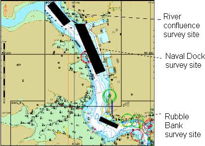
Fig 3c: Chart showing location of survey areas |
Successful grab samples were recovered at 50º23.24N, 04º11.71W and at 11.16 GMT, at the start of the 15 minute window either side of slack tide. The samples were collected to compare sediment type with the acoustic signal seen on the record. The second grab was taken along transect G9A08, 50º22.86N, 04º11.43W at 11:34.
After the seabed sampling, the vessel headed south to the Rubble Bank. The start of the transect was 50º21.86N, 04º11.86W and the end was at 50º21.90N, 04º11.15W by the third grab sample site (50º21.95N, 04º11.14W, at 12.06). However, the transect had to be cut short, due to the shipping lane being too busy. Instead, the vessel headed up to the confluence of the rivers Tamar and Lynher to commence some more transects. The first transect here started at 50º23.56N, 04º12.06W but was cut short because the water became too shallow at 4m, when the fish had to be recovered.
Results
The middle of the channel was composed mostly of coarse grained material. The greatest current flow occurs in the middle of the channel, which explains the lack of fine grained material which quickly becomes eroded away. Further, it is in the main part of the channel where most disturbance (resuspension) occurs due to the high shipping activity. There was evidence also of sediment mounds (highs) in the mid-channel close to the Naval Docks; one measured 70m in length and 50m in width. These could be the result of dredging activity to maintain the shipping channel.
The transects along the dredged area of the estuary, parallel to the dock wall, were less variable in their character and revealed the presence of fine-grained deposits. Generally, there is less turbulence and weaker currents along the edges of the estuary; thus fine-grained material is able to settle. Low current velocities along the edge of the dock walls are insufficient to disturb the material, for it to be washed away down the estuary.
There were indications of bedforms, possibly ephemeral near the dock walls. These were indistinct ripples, unable to form and stabilise due to constant disruptive tidal movements and turbulence created by propellers from ships.
|
Fig 3d: bifurcated wave ripples |
Some of the megaripples showed bifurcation (Fig 3d). This pattern is an indication of more than one current flowing, with current shear developing. Bifurcation in bedforms is indicative also of wave-dominated regimes. Bifurcation was found at the confluence of the two rivers, the Tamar and Lynher. Coarse grained material was found on the bed at the river confluence, where it had been transported down the rivers and brought into the estuary. Such coarse material could overly the fine grained sediments already present. Also, bedforms were present within medium grained sediments observed at this locality; these had an average wavelength of 2-3m. |
Anthropogenic factors can be identified using sidescan sonar e.g. dredging causing shallow channels and scouring in the bed. Coarse grained particles had accumulated around the corners of the dock wall, due to eddies created from the main current flow in the channel. Some cables and chains, of varying length but generally between 50-100m, were seen close to the river confluence.
The first grab sample (see above) revealed very fine grained oily mud with a light brown, very shallow overlying oxic layer with anthropogenic stone/cement clasts. The natural sediment is possibly of fluvial origin. The black anoxic layer formed the main bulk of the sample. The sediment in the second grab sample was mainly anoxic, with a very thin overlying oxic layer. Some bivalves were found at this site, as were slate and coal fragments; these probably originated from farther up the estuary. The sites for these two grab samples were used to 'calibrate' the sidescan record i.e. that low amounts of reflection were due to fine sediment, not to some discrepancy in the contrast setting of the instrument.
The third sample was taken from Rubble Bank. The sample was composed mainly of stone, rubble and biogenic material, which included mussel and cockle shells and many Crepidula fornicata. The surrounding sediments consisted of mud and fine sands. This sample site was selected as it showed a difference in the intensity of the acoustic reflection on the record, with more energy returning to the fish and indicating a harder substrate.
|
In terms of man-made structures, the resolution of the sidescan was sufficient to distinguish between wooden supports of part of the dock wall. Each support was approximately 40cm wide and, on the printout, they each appeared as individual structures (Fig 3e).
|
|
Offshore Data (X:\group9\Offshore data)
Using the survey ship Terschelling, the group undertook a transect consisting of 5 different stations from inside the Plymouth Sound breakwater to Eddystone Rock, approximately 19km offshore, on 25/06/04, between 08.00 and 16.00 GMT. The stations are shown in the chart (Fig.4.)
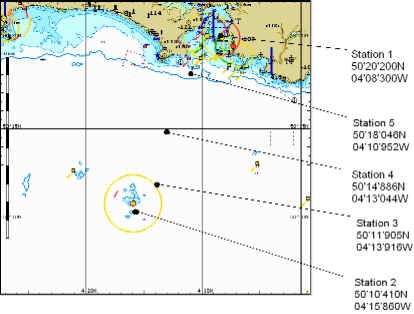
Fig.4: Chart displaying station positions.
This station is within the breakwater, and displayed a well-mixed vertical profile (Fig 4a), which is to be expected due to both the physical properties of the estuary topography (being shallow), and due to prevalent mixing processes, including tidal forces and wind mixing. Wind mixing was of particular importance on the day of sampling due to the weather conditions of the previous few days. The turbidity was increased as a result of this mixing; the 1% light depth was thus shallower than at any other station (Fig 4b).
|
|
Nutrient levels were generally low at this station, and thus are likely to be limiting to phytoplankton growth. Unusually, at this station phytoplankton numbers were higher at depth than in the surface waters, this is thought to be due to mixing of nutrients or phytoplankton cells in the water column previous to sampling. The dinoflagellate Noctiluca were present in the zooplankton net but not in phytoplankton counts as they are filtered out due to their large size. However, the low numbers of other smaller phytoplankton suggests that Noctiluca dominates the phytoplankton at this station. At this station copepods and hydrozoa dominated the zooplankton at the sampled depth of 0-7m suggesting a greater grazing control on phytoplankton at the surface.
Station 2 is located just to the south-east of Eddystone rocks (see chart). On the day of sampling, the development of a double thermocline was observed (Fig 4c), one at approximately 7-11m depth, the other at 11-20m. The seasonal and diurnal thermoclines identified are probably formed by solar heating of the surface layer by increased insolation.
|
|
The
presence of a double thermocline is thought to be due to the early stages of
reestablishment of stratification following previous mixing. Within the
lower thermocline, a deep chlorophyll maximum (DCM) was observed, which is
likely to be due to phytoplankton cells being present at an optimum for both
nutrients from below the thermocline, and light from the surface (Fig 4c).
However, the phytoplankton counts do not support this data: highest number of
cells per ml were observed in the upper thermocline at 4-5m depth. The 1%
light depth, or compensation depth, which is the base of the euphotic zone, was
found to be deepest at station 2 (Fig
4b),
possibly indicating low turbidity. In the zooplankton, copepods and
hydrozoa again dominated in the two vertical net trawls which were taken from
40m to the surface. However, compared to station 1, there were low
densities of the dinoflagellates Noctiluca and Ceratium, although
other phytoplankton densities were higher at this station than any other.
Nutrient concentrations (phosphate, nitrate and silicate) were much lower than at stations further inshore, likely to be due to reduced levels of riverine and terrestrial input and the effect of high phytoplankton abundances. Dissolved oxygen was higher in the surface waters in comparison to other stations, this is reflected in the high numbers of phytoplankton cells. In Fig 4c, the CTD recorded an unavoidably high level of salinity spiking which could not be smoothed from the data thus the data plotted is unrefined. |
Again, there was found to be a double thermocline at this station, although the lower thermocline, at 25-30m, was less well developed than at station 2 or the upper thermocline at 3-4m. A DCM was observed at 35m depth, just below the lower thermocline. Interestingly, also at this depth there was found to be a peak in dissolved oxygen. Figure 4d shows that phytoplankton densities were maximal at both 5m (which coincides with depleted nitrate concentrations) and 25m (corresponding with depleted silica concentrations): the deeper peak is likely to be responsible for the observed features above. However, the phytoplankton counts, which were dominated by diatoms, revealed there to be lower cell numbers than at the other stations. Despite this, in the zooplankton samples the dinoflagellates Noctiluca and Ceratium were present in very high densities and thus dominated the overall plankton community (Fig 4e, 4f). It seems likely that Ceratium outcompetes the other autotrophic phytoplankton (Noctiluca is heterotrophic) thus forming a bloom at this station. The peak in chlorophyll and dissolved oxygen at depth is likely to be due to this bloom.
 |
 |
|
The temperature transect between Station 2 and Station 3 (Fig 4g) clearly
shows the progressive appearance of strong thermal gradients as
Terschelling approaches Plymouth Sound. In fact, this feature can be
broken down into two components, a seasonal thermocline and a diurnal
thermocline caused by solar heating of the surface layer. These features
can also be recognized in Confidence in resolution of the two thermal features is high as the Minibat made several passes through the water column in this location. |
Fig 4g: Minibat temperature transect |
|
The fluorescence data (Fig 4h) clearly shows two areas of high chlorophyll concentration just off station 2 at thirteen metres and another feature of lesser concentration appears between 6-8m depth. The deep feature is represented as a peak in the CTD fluorometer data and the chlorophyll concentration data however is absent in the phytoplankton counts. By contrast, the shallow feature is not displayed in the CTD data, but appears as a strong peak in the phytoplankton counts. Again, the resolution of these features is good as the Minibat was guided through these regions on several occasions. |
Fig 4h: Minibat chlorophyll fluorescence transect |
This station, close to the breakwater (see chart of locations) showed some evidence of a thermocline at 6-11m but this was not very well defined. The nutrient profiles also displayed characteristics of a well-mixed water column with concentrations being relatively low and approximately constant with depth. Phytoplankton counts at this station displayed the same trend as station 1 with number of cells per ml being greatest below 20m (counts of 50 cells/ml) compared to surface waters (counts of 10 cells/ml at 5m). The zooplankton net was used between 7m and the surface and no Ceratium were found in the sample supporting the low numbers of autotrophs observed. The turbulence of the water column would help to explain the low numbers of dinoflagellates and dominance of diatoms at this station. The zooplankton community was again dominated by copepods and hydrozoa, with some other taxa such as appendicularians and decapod larvae present in higher abundance than at other stations.
Acoustic Doppler Current Profiler (ADCP) Analysis:
The ADCP highlights the amount of suspended particulate matter present within a certain water body. Through analysis of the backscatter collected at the five stations, Minibat transects and Richardson number calculations, the extent of shear turbulence of the water column can be inferred.
The Richardson number for Station 1 at a depth of 6m was found to be 74.183 thus reflecting stable, laminar flow. The average backscatter profile (Fig 4j) shows a strong reflection at the bottom which is possibly a resulting factor of the turbulent weather conditions of the preceding days. Since this station is in fact behind the breakwater, the conditions are expected to be statically stable in comparison with Fig 4k below. The surface waters show a relatively high concentration of zooplankton which could correlate with the strong reflectance patterns shown on the profile below.
Fig4j: ADCP average backscatter profiles for Station 1.
Fig 4k below combines backscatter images for both stations 2 (left hand side) and 3 (right-hand side of the image). The area of high reflectance in the upper water column of station 2 agrees when compared with the phytoplankton samples taken. This hypothesis is also supported by the ideas put forward from both Minibat and Fluorometer readings. The inclined sea floor at station 2 (figure 4l) is the root of the strong reflections at the seabed.
Station 3 is the point at which the seasonal and diurnal thermoclines were identified as formed by solar heating of the surface. This input of heat reduces the density of the surface layer thus increasing the overall stability shown by the very high Richardson number at 4m (Ri = 341.689). Considering the Minibat temperature profile (Fig.4g) a strong temperature gradient can be seen at similar depths, reinforcing the inference of a thermocline. The profile below shows that in the surface depths, there is a band of high reflectance, which could be the result of either density differences, chlorophyll concentrations, or phytoplankton blooms which all show a general increase in our collected results. Below the initial thermocline, at 4m, there is another zone of high reflectance as Ri turns from 0.457 at 6m to 7.559 at 8m. This could correspond to suppressed vertical mixing of the benthic sediments as can be seen on the profile.
Fig 4k: ADCP average backscatter profiles for stations 2 and 3.
Previous and current data collected at station L4 (50o15'N 4o13'W)
Previous and current data for Noctiluca and Ceratium at station L4
OFFSHORE TERSCHELLING
| Station | Time/GMT | Date | Position/GPS |
| 1 | 8.42 | 25/06/2004 | 50°20.27N |
| 004°08.39W | |||
| 2 | 11.20 | 25/06/2004 | 50°10.41N |
| 004°15.86W | |||
| 3 | 13.10 | 25/06/2004 | 50°11.905N |
| 004°13.916W | |||
| 4 | 14.04 | 25/06/2004 | 50°14.886N |
| 004°13.004W | |||
| 5 | 15.14 | 25/06/2004 | 50°18.046N |
| 004°10.952W |
ESTUARINE BILL CONWAY
| Station | Time/GMT | Date | Position/GPS |
| 1 | 9.00 | 05/07/2004 | 50°20.139N |
| 004°10.093W | |||
| 2 | 9.40 | 05/07/2004 | 50°20.149N |
| 004°08.080W | |||
| 3 | 10.10 | 05/07/2004 | 50°21.664N |
| 004°08.193W | |||
| 4 | 11.14 | 05/07/2004 | 50°24.037N |
| 004°12.433W | |||
| 5 | 11.37 | 05/07/2004 | 50°23.515N |
| 004°12.236W | |||
| 6 | 12.03 | 05/07/2004 | 50°23.798N |
| 004°12.943W | |||
| 7 | 12.50 | 05/07/2004 | 50°24.579N |
| 004°12.236W | |||
| 8 | 13.32 | 05/07/2004 | 50°21.671N |
| 004°10.251W |
ESTUARINE RIB
| Station | Time/GMT | Date | Positions/GPS |
| 1 | 10.31 | 28/06/2004 | 50°29.750N |
| 004°12.411W | |||
| 2 | 11.21 | 28/06/2004 | 50°29.732N |
| 004°12.412W | |||
| 3 | 11.31 | 28/06/2004 | 50°29.784N |
| 004°12.575W | |||
| 4 | 11.44 | 28/06/2004 | 50°29.836N |
| 004°12.775W | |||
| 5 | 11.46 | 28/06/2004 | 50°29.866N |
| 004°13.014W | |||
| 6 | 12 | 28/06/2004 | 50°29.886N |
| 004°13.261W | |||
| 7 | 12.21 | 28/06/2004 | 50°29.604N |
| 004°13.246W | |||
| 8 | 12.29 | 28/06/2004 | 50°29.258N |
| 004°13.370W | |||
| 9 | 12.43 | 28/06/2004 | 50°28.766N |
| 004°13.051W | |||
| 10 | 13 | 28/06/2004 | 50°28.651N |
| 004°13.048W | |||
| 11 | 13.1 | 28/06/2004 | 50°28.598N |
| 004°13.091W | |||
| 12 | 13.17 | 28/06/2004 | 50°28.063N |
| 004°14.134W | |||
| 13 | 13.34 | 28/06/2004 | 50°27.539N |
| 004°14.240W | |||
| 14 | 13.46 | 28/06/2004 | 50°27.792N |
| 004°13.518W | |||
| 15 | 14 | 28/06/2004 | 50°27.611N |
| 004°12.541W | |||
| 16 | 14.13 | 28/06/2004 | 50°27.072N |
| 004°12.343N | |||
| 17 | 14.32 | 28/06/2004 | 50°24.559N |
| 004°12.201W |
GEOPHYSICS
| Transect | Date | Start of line time/GMT | Start Position/GPS | End of line time/GMT | End Position/GPS |
| 1 | 02/072004 | 9.33 | 50°22.76N | 9.45 | 50°23.39N |
| 004°11.16W | 004°11.66W | ||||
| 2 | 02/072004 | 9.47 | 50°23.40N | 9.55 | 50°22.74N |
| 004°11.60W | 004°11.13W | ||||
| 3 | 02/072004 | 9.58 | 50°22.81N | 10.08 | 50°23.41N |
| 004°11.18W | 004°11.59W | ||||
| 4 | 02/072004 | 10.11 | 50°23.39N | 10.19 | 50°22.73N |
| 004°11.60W | 004°11.19W | ||||
| 5 | 02/072004 | 10.21 | 50°22.37N | 10.33 | 50°23.36N |
| 004°11.26W | 004°11.75W | ||||
| 6 | 02/072004 | 10.35 | 50°23.34N | 10.43 | 50°22.73N |
| 004°11.77W | 004°11.29W | ||||
| 7 | 02/072004 | 10.54 | 50°22.71N | 11.04 | 50°23.39N |
| 004°11.32W | 004°11.86W | ||||
| 8 | 02/072004 | 12.22 | 50°21.86N | 12.25 | 50°21.96N |
| 004°10.86W | 004°11.15W | ||||
| 9 | 02/072004 | 12.39 | 50°21.85N | 12.41 | 50°21.95N |
| 004°11.05W | 004°11.29W | ||||
| 10 | 02/072004 | 12.51 | 50°22.71N | 12.57 | 50°23.23N |
| 004°11.37W | 004°11.78W | ||||
| 11 | 02/072004 | 13.08 | 50°23.90N | 13.13 | 50°23.51N |
| 004°12.47W | 004°12.12W | ||||
| 12 | 02/072004 | 13.15 | 50.23.52N | 13.17 | 50°23.65N |
| 004°12.17W | 004°12.30W |
Sediment Grabs
| Date | Time/GMT | Position/GPS | |
| 1 | 02/07/2004 | 11.16 | 50°23.24N |
| 004°11.71W | |||
| 2 | 02/07/2004 | 11.34 | 50°22.86N |
| 004°11.43W | |||
| 3 | 02/07/2004 | 12.08 | 50°21.92N |
| 004°11.18W |
Disclaimer: This web site represents the work of group 9 only, and the data do not in any way reflect the views of the University of Southampton or the Southampton Oceanography Centre.