
This is the ADCP data interpretation section of the group 8
website. ADCP data were taken on both
research vessel Terschelling
and the Bill Conway.

TRANSECT 1
STATION 1 -2
(g8adcposhore001.000)
|
Start |
|
|
End |
|
|
|
Time |
Lat. |
Long. |
Time |
Lat. |
Long |
|
1016 |
50°20.055 |
04°07.950 |
1146 |
50°11.206 |
04°14.064 |
This transect begins at station 1 located near the breakwater, it then
continues out to station two located near the
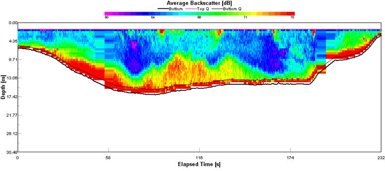
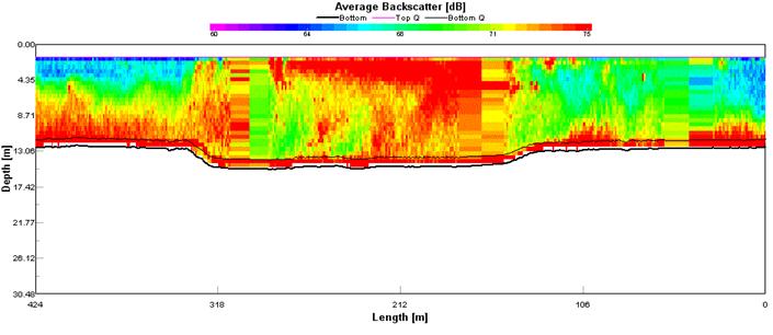
A high backscatter return is seen at the surface along this
transect. This is most likely a result
of the turbulence and mixing caused by the vessels movement through the
water. Regions of patchy seaweed and
surf may also add to the high return. At
depth 35m, the backscatter and velocity magnitude data give a false reading and
should be ignored.
There is a region of medium backscatter as the
transect leaves the Sound with seabed depth 14m. Throughout the transect patches of high
backscatter (64dB) are evident between 8 and 30m.
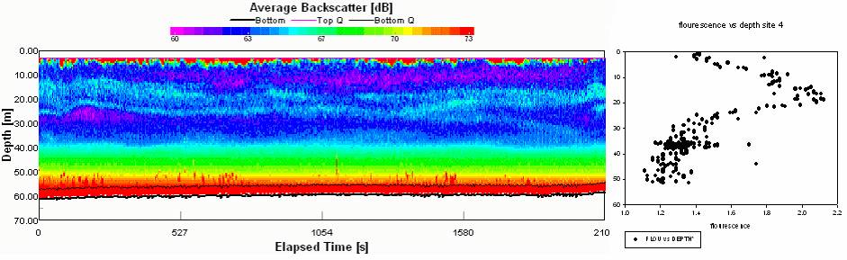
Throughout the transect there is a distinct
band of high backscatter between 6 and 14m shaded light blue/green. This information can be compared to the fluorescence
reading taken with the CTD at the end of the transect (station 2). The fluorometer
measures the photosynthetic activity of the phytoplankton, this
ranges from 11 to 24. When the
two profiles are placed next to one another it is evident that the high
backscatter between 6 and 14m is related to phytoplankton in that region of the
water column. This can also be related
to the thermocline.
This is due to the low level of nutrients in the surface waters owing to
plankton blooms in the weeks leading up to this survey. The plankton have
dropped down to the base of the thermocline towards
the limits of the euphotic zone. The plankton are
able to utilise the nutrients present both above and below the thermocline in this area.
----------------------------------------------------------------------------------------------------------------------------------------------------------------------------------------------------
TRANSECT 2 STATION 2-3
(g8adcposhore002r.000)
|
Start |
|
|
End |
|
|
|
Time |
Lat. |
Long. |
Time |
Lat. |
Long |
|
1222 |
50°11.200 |
04°14.115 |
1308 |
50°10.188 |
04°16.032 |
This transect shows patchy areas of
backscatter between the surface and 40m (71dB), but mainly 68dB areas of low
backscatter.
----------------------------------------------------------------------------------------------------------------------------------------------------------------------------------------------------
TRANSECT 3 STATION 3
(g8adcposhore004r.000)
|
Start |
|
|
End |
|
|
|
Time |
Lat. |
Long. |
Time |
Lat. |
Long |
|
1222 |
50°10.180 |
04°16.030 |
1308 |
50°11.709 |
04°18.329 |
.
This transect shows the base of a large feature on the seafloor, this is
part of the Eddystone Rock. Velocity magnitude remains constant for much
of the profile, however where the rock is at its highest, it is influencing the
velocity magnitude of the water column, increasing flow by 0.3m/s to 0.4m/s.
The geological feature is strongly influencing the thermocline
and general profile of the water column either side of it. There is low backscatter seen directly above
the rock between 10m and 30m. This is a
result of bottom water being pushed up higher into the water column as it flows
past the
----------------------------------------------------------------------------------------------------------------------------------------------------------------------------------------------------
TRANSECT 4
STATION 3 -4 (g8adcposhore003r.000)
|
Start |
|
|
End |
|
|
|
Time |
Lat. |
Long. |
Time |
Lat. |
Long |
|
1308 |
50°10.180 |
04°16.030 |
1344 |
50°11.709 |
04°18.329 |
This transect shows high backscatter at
the surface, with choppy turbulent waters at 4-5 metres depths. There is a band of low backscatter that
fluctuates between 16m and 25m across the whole transect. At the start of the
transect the backscatter is high at the surface, this area of high
backscatter then extends down into the water a further ten metres. In doing so it pushes the band of low
backscatter further down the water column profile. Where the high backscatter extends down into
the water column, very high backscatter readings associated with rough seas and
the movement of the survey vessel can be seen at the surface. These features may therefore represent the
pitching and rolling of the vessel. It may
also be a result of turbulence caused wind at the air sea interface.
----------------------------------------------------------------------------------------------------------------------------------------------------------------------------------------------------
TRANSECT 5
STATION 4
(g8adcposhore005.r000)
|
Start |
|
|
End |
|
|
|
Time |
Lat. |
Long. |
Time |
Lat. |
Long |
|
1436 |
50°11.986 |
04°17.776 |
1511 |
50°11.959 |
04°18.213 |
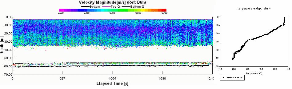
These two transect profiles show a banded water column. Similarly to Transect 1, a band of photosynthetically active organisms is found between depths 10m and 25m. This again is backed up by graphs of fluorescence
and the thermocline, that show three distinct layers within the water
column. Phytoplankton and zooplankton
can be found at the base of the thermocline. One can refer to pie charts of the
zooplankton community to confirm this statement.
It can be concluded that marine plankton and organisms can be found in
their greatest concentrations near the base of the thermocline,
around the
----------------------------------------------------------------------------------------------------------------------------------------------------------------------------------------------------

|
Transect |
Start |
|
|
End |
|
|
|
|
Time |
Lat. |
Long. |
Time |
Lat. |
Long |
|
0853 |
50°20.554 |
4°10.054 |
0909 |
50°20.575 |
4°07.799 |
|
|
2 |
0910 |
50°20.575 |
4°07.799 |
0917 |
50°20.038 |
4°08.194 |
|
3 |
0933 |
50°20.166 |
4°08.195 |
0945 |
50°20.154 |
4°09.574 |
|
4 |
0950 |
50°20.103 |
4°09.628 |
0957 |
50°20.515 |
4°10.113 |
|
5 |
1021 |
50°21.579 |
4°10.060 |
1024 |
50°21.518 |
4°10.236 |
|
1046 |
50°21.577 |
4°10.147 |
1050 |
50°21.589 |
4°10.136 |
|
|
7 |
1051 |
50°21.618 |
4°10.054 |
1054 |
50°21.514 |
4°10.245 |
|
1130 |
50°24.430 |
4°12.322 |
1133 |
50°24.426 |
4°12.115 |
|
|
9 |
1206 |
50°23.990 |
4°12.342 |
1209 |
50°23.989 |
4°12.662 |
|
1210 |
50°24.002 |
4°12.643 |
1215 |
50°23.575 |
4°12.611 |
|
|
11 |
1217 |
50°23.563 |
4°12.516 |
1220 |
50°23.794 |
4°12.282 |
|
1240 |
50°23.854 |
4°12.426 |
1243 |
50°23.671 |
4°12.297 |
|
|
13 |
1245 |
50°23.732 |
4°12.364 |
1249 |
50°23.792 |
4°12.378 |
|
1324 |
50°23.046 |
4°11.886 |
1328 |
50°23.179 |
4°11.415 |
Click this
link to access a readme file covering the processed
transect data
|
Start |
|
|
End |
|
|
|
Time |
Lat. |
Long. |
Time |
Lat. |
Long |
|
0853 |
50°20.554 |
4°10.054 |
0909 |
50°20.575 |
4°07.799 |
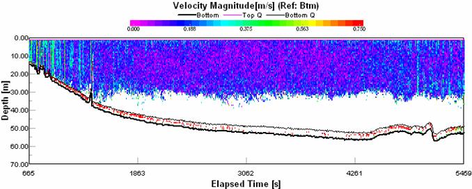
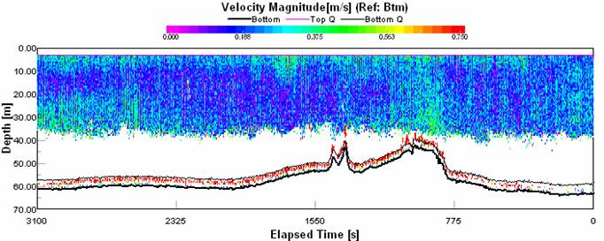
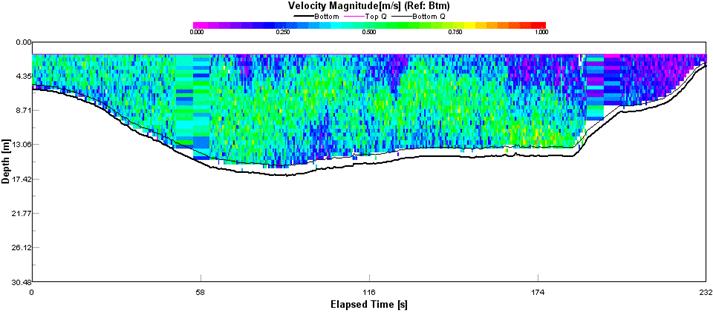
This was the first ADCP transect taken and perhaps the most
exciting. The transect
is divided into two sections, vertical banding and horizontal banding. The vertical banding on the left hand side of
the plot depicts eddying within the water column up until 150secs into the
transect.. This
is caused by the headland that protrudes into the Sound. This strongly influences any water mass that
passes it, creating eddies. The
influence of the headland soon diminishes as the vertical banding is converted
into horizontal banding. This shows that
water below 5m is flowing into the Sound whereas water above this point is
moving with the ebbing tide.
----------------------------------------------------------------------------------------------------------------------------------------------------------------------------------------------------
|
Start |
|
|
End |
|
|
|
Time |
Lat. |
Long. |
Time |
Lat. |
Long |
|
1046 |
50°21.577 |
4°10.147 |
1050 |
50°21.589 |
4°10.136 |
This plot was taken in the “Narrows” as an accompaniment to the CTD profile taken. The area of water measured was actually very small,
as the vessel was allowed to drift with the current whilst the CTD was
deployed. As this measures over the
duration of the CTD deployment a clear profile of the water column can be seen. Water between 10m and 20m can be seen
entering the River Tamar on a bearing of 290° to 310°, despite it being
15minutes after low tide at Devonport.
A flux of water can be seen leaving at the surface the River Tamar and
heading out into the Sound. This creates
the horizontal banding also seen in Transect 1.
----------------------------------------------------------------------------------------------------------------------------------------------------------------------------------------------------
|
Start |
|
|
End |
|
|
|
Time |
Lat. |
Long. |
Time |
Lat. |
Long |
|
1130 |
50°24.430 |
4°12.322 |
1133 |
50°24.426 |
4°12.115 |
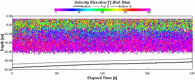
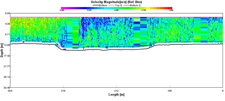
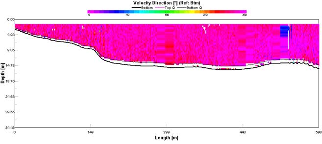
This ADCP profile shows variation in the velocity magnitude seen in the
Tamar. The velocity magnitude is seen to
increase at the base of the profile.
This can be related to the asymmetric channel profile. Where the depth of water is at its most
shallow, at 0 time, velocity equals 0.4m/s.
it then decreases as the channel deepens. A sharp increase in velocity is shown in
green. This is at its greatest where the
channel morphology changes, from a flat bottom to a cliff. This may be due to the thalweg
of the river, taking the most efficient path down river. The features seen here, tie in with the
erosion and depositional features seen in river and estuarine systems. The flow direction is between 300° and 025°
degrees indicating an incoming tide.
----------------------------------------------------------------------------------------------------------------------------------------------------------------------------------------------------
|
Start |
|
|
End |
|
|
|
Time |
Lat. |
Long. |
Time |
Lat. |
Long |
|
1210 |
50°24.002 |
4°12.643 |
1215 |
50°23.575 |
4°12.611 |
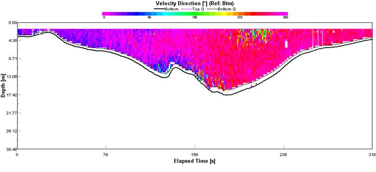
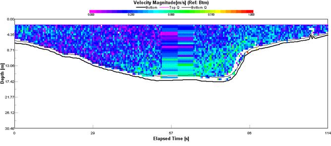
This transect shows an interesting surface
feature found between 196 and 240 seconds. This ranges from surface to a depth
of 4.9m. This water mass is travelling
at a very low velocity between 0 and 0.2 m/s.
it is also flow in the opposite direction as
can be seen in the velocity direction profile. This again is a low flow feature when compared
to the rest of the transect. Water velocity remains at its greatest in the
shallow region of the estuary, between 0.5 and 0.7 m/s.
----------------------------------------------------------------------------------------------------------------------------------------------------------------------------------------------------
|
Start |
|
|
End |
|
|
|
Time |
Lat. |
Long. |
Time |
Lat. |
Long |
|
1217 |
50°23.563 |
4°12.516 |
1220 |
50°23.794 |
4°12.282 |
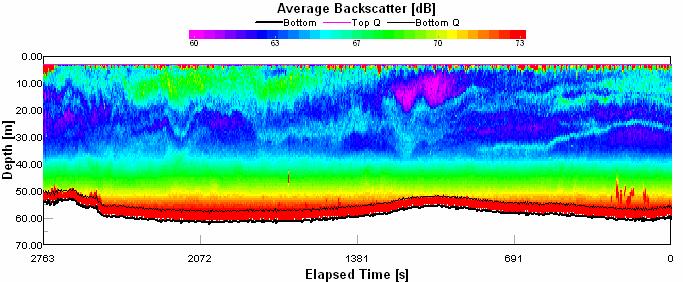
In this transect, average backscatter and velocity magnitude can be
compared. These two profiles show a
correlation between the velocity of a body of water and the amount of
backscatter produced. At this point, a
low velocity is reflected by a high backscatter reading.
These features could also be seen with the naked eye when observing the
water surface from the vessel.
Surface features shown here in the centre of the transect, may be the
result of mixing caused by vessels passing up and down the river. The propellers and wake will cause mixing in
the water column as well as increasing turbidity. This will alter the backscatter, flow
velocity and the direction of flow. Transect 14 shows an example of the effect that river
traffic has on the ADCP transect.
----------------------------------------------------------------------------------------------------------------------------------------------------------------------------------------------------
|
Transect |
Start |
|
|
End |
|
|
|
|
Time |
Lat. |
Long. |
Time |
Lat. |
Long |
|
12 |
1240 |
50°23.854 |
4°12.426 |
1243 |
50°23.671 |
4°12.297 |
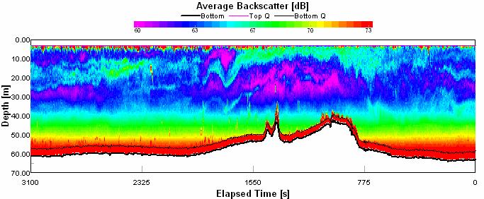
Whilst en route to station 10 a front system could be seen at the
surface of the estuary. The CTD system
was deployed, and the vessel drifted (engines off) through the front. During the CTD sampling, the ADCP data was
recorded. This shows alternating bands
of water at the surface. The fronts were visible as a result of the lack of
water movement at the surface. The comparative
calm could easily be distinguished from the more turbulent estuarine
waves. The backscatter
transect makes defining the different fronts easier. The low velocity bands of water have a high
turbidity, and therefore backscatter reading when compared to the faster
flowing low backscatter water seen either side of the front, (middle of transect). Horizontal banding can be seen at the left of
the transect. This
however is not reflected in the velocity direction data, meaning that flow
velocity is most likely dependent on friction with the bottom.
----------------------------------------------------------------------------------------------------------------------------------------------------------------------------------------------------
|
Transect |
Start |
|
|
End |
|
|
|
|
Time |
Lat. |
Long. |
Time |
Lat. |
Long |
|
14 |
1324 |
50°23.046 |
4°11.886 |
1328 |
50°23.179 |
4°11.415 |
This transect shows the influence that a passing vessel can have on the
ADCP data retrieved. The vessel passed
in front of the Bill Conway in mid transect.
The distinct blue feature extending to a 5m depth is a result of the
wake and turbulence produced by the boat
hull and propellers as it passes through the water.