Plymouth 2004

Group 4

Back - David Mans, Suzi Buchan, Mike Brewer, Crystal Szczerbicka, Simon du Boulay, Robert Lancaster
Front - Eleonora Manca, Luke Aki

Contents

• Introduction
• Geophysics   26/06/04
• Lower Estuarine Work  29/06/04 
• Offshore Work  03/07/04
• Upper Estuarine Work 06/07/04
• Appendix 

Introduction

    The River Tamar and Plymouth Sound was the subject of a multidisciplinary study into the biology, physics and chemistry of the area. The River Tamar extends for some 31km and has a catchment area of 1700 km² (Evans et al. 1993). The Tamar is a partially mixed macrotidal estuary and can be classed as a Ria. Four separate days were spent surveying the upper, lower and offshore parts of the estuary.  One of these days consisted of a geophysical survey of the mid-part of the estuary.                                                                                

1. Upper Estuarine Work		3. Geophysical Survey
2. Lower Estuarine Work		4. Offshore Sampling

Figure 1 - Map showing locations of sampling.

Back to Top

References:

Evans K.M., Fileman T.W., Ahelm, M., Mantoura, R., and Cummings, D., 1993, Fate of organic micropollutants in estuaries (triazine herbicides and alkyl phenol polyethoxylates). National Rivers Authority.

---

Geophysical Survey of the Lower Tamar Estuary                                      

    1.1 Introduction
    1.2 Transect and Tidal Information                                    
    1.2 Analysis                       
    1.3 References

    Back to Top

1.1 Introduction 

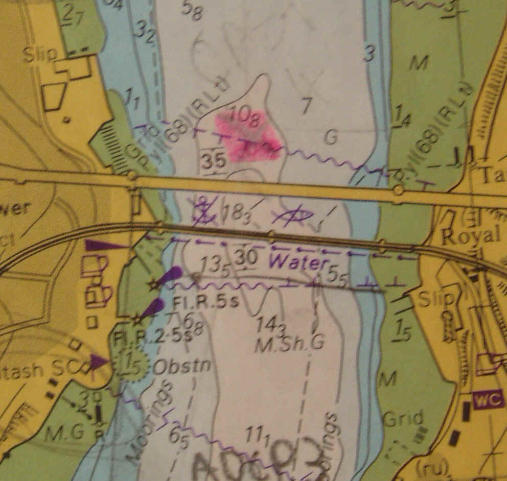
    An area of the River Tamar, extending from the Tamar Bridge to the Ocean Court Marina, was surveyed by side-scan sonar. It was carried out on board the Nat West II research vessel. The investigation was intended as a combined study of river  bedforms, anthropogenic activity and dock wall construction type. Side-scan sonar (Figure 3) operates using sound pulses of either 100 and 500 KHz. A higher frequency provides better resolution, but less penetration. These sound pulses are transmitted and the return echo measured to generate a ‘picture’ of the sea floor. By a process of trial and error, a 500 KHz frequency was deemed to produce the clearest image of the estuary bed.
    Three transects were selected; 1) centred on the Royal Albert Bridge; 2) around the north west corner of HMS Drake; 3) along south side of HMS Drake dock wall. A towed fish, with the side-scan sonar transmitter and receiver mounted within in it, was lowered over the rear of the vessel for each of the transects. The fish was aimed to be towed at an average of 4 knots and was towed at 1 metre below the surface. Two methods were used to record the data. A hard copy was produced using a more dated side-scan sonar receiver linked to a paper plotter. A computer-based system was used also, providing a link between position, time and speed.  
    In order to calibrate the instruments, a Van Veen grab was used to take a sediment sample at grid square 565441. This was compared to the image produced by the side-scan sonar to confirm the sediment types. A fine mud was brought up by the grab producing a light side-scan sonar image. Therefore, darker images indicated coarser sediment types such as gravels and bed rock; lighter images indicate silts and very fine muds.    

  Back to Geophysics Contents



1.2 Transect and Tidal Information
       1.2.1 Tidal Information
       1.2.2 Transect information

 

1.3 Analysis of the geophysics surveys     The printouts were analysed and the major features were recorded and measured. Isometric plots were produced using the position data acquired from the ships GPS. The regions of major features such as exposed bedrock, sand ripples or (man-made) bridge supports were then noted.   1.3.1 Area surrounding Royal Albert Bridge     On the first transect, between 58000 and 59000 Northings, and from 243200 to 243600 Eastings, bifurcated bedforms (megaripples) were identified, which extended for a length of 54m.  These appeared to show a wave-dominated system, as opposed to a tidally-dominated system. On the eastern side, the average wavelengths of these features were 9m, which compared to 18m on the western side, possibly due to less wave-dominated energy on the eastern side. This difference in energy between these two banks could explain also why the sediment is coarser on the eastern side, where the bedforms have a shorter wavelength and are finer-grained than on the western side.     Between 58600 and 58800 Northings, bridge supports showed up on the side-scan sonar. On either side of these supports there were no sand waves apparent, due to turbulence and eddies that are induced by contact of the supports with tidal currents.  Behind the eastern bridge support the bedrock is evidently more exposed than elsewhere. This bedrock is covered with fine sediment on either side of the western bridge support. 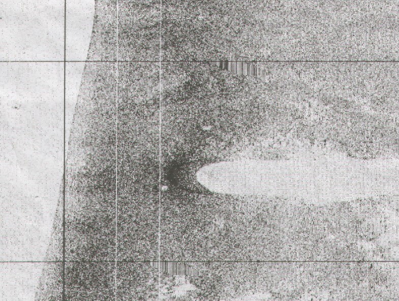On this bedrock there is evidence of anthropogenic activity, as illustrated by the construction of bridge supports and piers. Further south, between 58200 and 58400 Northings, there is further evidence of anthropogenic activity in the form of mooring lines that extend for a length of 630 m. Associated with these mooring lines is a zone of sediment striping, which could indicate dredging activity.

Figure 2 - Side scan print out of the dock wall.

Figure 3 : A chart showing the location of the 1st transects.	Figure 4 :  An isometric plot of the area centred around  Royal Albert Bridge.	Figure 5 : A sidescan print out of Royal Albert Bridge.

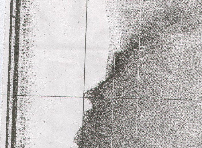
1.3.2 North West Corner, near by HMS Drake

    The second transect was between 55600 and 56400 Northings, and 243800 and 244600 Eastings. This revealed a scour mark, possibly due to the intersection of the River Tamar and the River Lynher, between 55600 and 55800 Northings.

    The only other point of interest is an area of faint dredge marks, observed between 56200 and 56000 Northings. Otherwise, the bed is uniform in terms of sediment type, with no further evidence of bedforms or anthropogenic activity. 

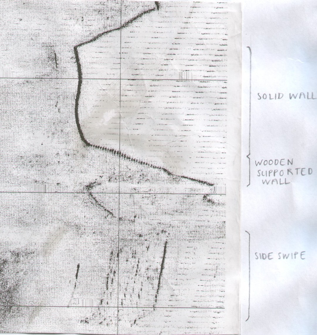
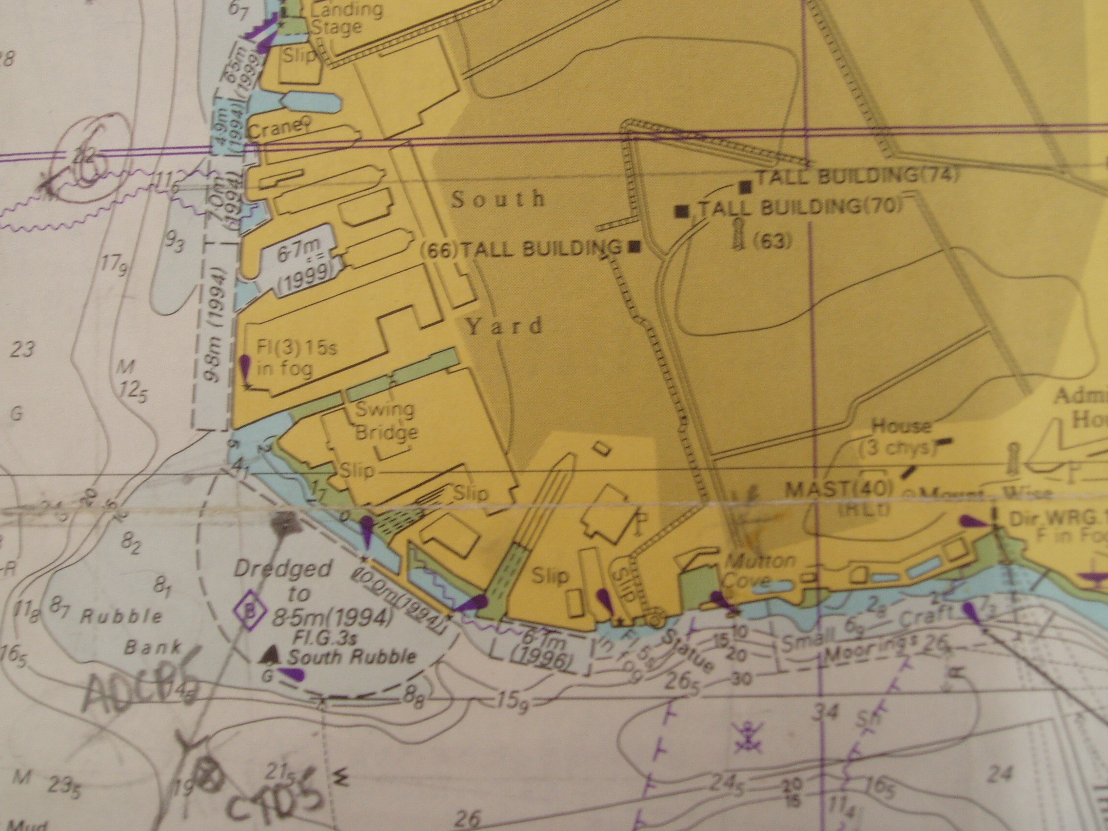
1.3.3 Southern Dock Wall
    The third and final transect was used to test the effectiveness of the side-scan sonar at detecting different materials used in the construction of the docks. The transect lies between 54000 and 55000 Northings and 244600 and 245000 Eastings. This area is located near the Southern Dock wall. The resulting plot enables some differentiation between a solid concrete wall and a wooden supported wall. On the side-scan sonar printout there is evidence of side swipe, which indicates reverberation from a thick concrete structure, this gives off several reflections of the sound pulse.

Figure 6 : A chart showing the section of Dock Wall surveyed.	Figure 7 : A sonograph print identifying a scour mark.	Figure 8 : A picture showing the grab  sample.

    From the surveys it is evident that this form of data is not of sufficient detail to make firm conclusions about dock wall construction. However we have shown that it may be useful for identifying areas where further investigation would be beneficial using other means such as divers. It has also been shown that the side scan sonar is more suited to identifying larger bedforms and sediment types on a river or seabed.  

1.3.4 Grab results
    The grab was taken at 50º 23'052N, 4º 11'162W, and confirmed the sediment type predicted from the print out. The sediment consisted of fine material with a thin surface oxic layer. The grab also contained a number of angular rocks.     

    A number of problems were experienced while taking the transects:

•        Ideally the transects are conducted in a straight line and at the same speed, this enables maximum coverage. In a busy estuary, however, with other water users and moorings present, it is unavoidable that there are turns in the transects. The change of speed and direction created problems when the transects were lined up side by side. The overlap produced repetition of scanning. The change of speed created "stretching" of data as the the printer was still working at the same speed.
•       The location of the fish was different  from the GPS reading taken on the boat, as the GPS receiver was near the cabin and the fish was towed behind. This has resulted in the locations plotted on the isometric plot being out by the distance between the two. The GPS satellite signal was often blocked as the boat travelled under the bridge, meaning it was difficult to keep track of the correct line.

1.1.4 References
www.tamarvalley.org.uk
www.tamarvalleytourism.co.uk
www.tamarbridge.org.uk

Jones, G.E. & Glegg, G.E., 2004, Effective use of geophysical sensors for marine environmental assessment and habitat mapping, WIT Press, www.witpress.com

Back to Top

 

---

Samples of the Lower Estuary (Bill Conway)
2.1 Introduction 2.2 Position Data 2.3 Analysis 2.4 Summary 2.5 References Back to Top
		R.V Bill Conway

2.1 Introduction

Aim - The aim of this research was to observe how the Tamar estuary acts as an interface between low salinity river water and high salinity sea water together with its effect on the chemistry of the estuary. 

    Results are presented from a survey carried out on the RV Bill Conway on the 29^th June 2004 . The purpose of the study was to examine the biological, chemical and physical characteristics of the Tamar Estuary to determine if the typical profile expected of riverine estuaries of this kind  is evident. The focus was on the expected conservative behaviour of major nutrients and aquatic components of estuaries (chlorophyll, nitrates, silicates, oxygen and phosphates).  The research was carried out with the use of an (Acoustic Doppler Current Profiler (ADCP) and CTD with rosette bottles attached.  Samples were taken at the surface, mid-depth and at the base of the water column, at selected sites.  The survey took place between 50°24’225, 4°12’290 (just north of Ernesettle Pier) and 50°20’500, 4°10’160 (Plymouth Breakwater) and included 11 sites.

 

    The study was carried moving downriver against an incoming tide. The 11 sites were selected for sampling and study, as the result of being either at a confluence of rivers or at a point where flow would be definitive of flow patterns occurring within a chosen transect. The flow patterns at these transects were mapped using an ADCP. Where surface evidence of water column stratification was present along a transect a CTD was cast and water sample collections were undertaken. Two horizontal plankton net samples, with a mesh size of 200µm, were also taken during the course of the survey, one in the upper part of the survey and one out to sea, near the breakwater.

                                                                                                Chart 1 - Position of the 11 stations visited on the Bill Conway.
2.2 Position Data + Tidal data
     2.2.1 Tide Information
      2.2.2 ADCP Data
      2.2.3 CTD Data
      2.2.4 Plankton

2.3 Analysis
       2.3.1 ADCP
      2.3.2 CTD
      2.3.3  Nutrients
      2.3.4 Oxygen
      2.3.5  Chlorophyll
      2.3.5  Zooplankton

 2.3.1 ADCP Data

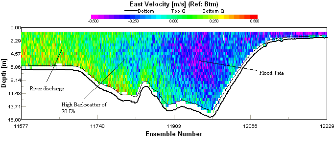
    At the confluence of the River Lynher and Tamar, three transects were taken using the ADCP.  The transects were taken on a flood tide. It was found that river water flowed outwards along the northern edge of the River Lynher, whereas the sea water was found along the southern deeper side.  Furthermore, a large amount of backscatter (Tattersall et al, 2003) was observed where the two water bodies met.  This backscatter was indicative of turbulent mixing (Figure 9).

	Figure 9 - Velocity of water travelling in an easterly direction across the River Lynher.

    The flood tide observed entering the River Tamar behaved in the expected manner, in terms of an evident northward flow, with the denser seawater moving below the lighter freshwater (except that it had been pushed eastwards by the freshwater flow from the River Lynher) (Uncles & Lewis, 2001). At West Mud buoy, a large eddy was observed moving in an anticlockwise direction into Saint Johns Lake, as shown by the alternating green and blue contour in Figure 10.
 

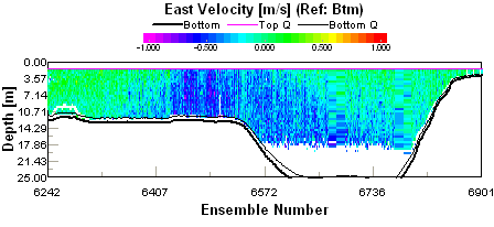
	Figure 10 - Velocity of water travelling in an easterly direction from West Mud Buoy to Plymouth Docks.

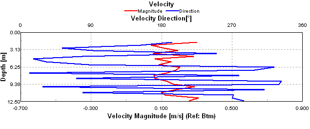
    The likely cause of the eddy is the presence of the dock walls north of the narrows.  The dock walls divert the flow into Saint Johns Lake, where the area is sufficiently large enough to allow the eddy to form. This eddying presents itself in the ADCP record as a series of directional switches in direction of flow (Figure 11), further evidence is seen in the backscatter data.

 

	Figure 11 - A graph of flow direction and magnitude illustrating the eddying around West Mud Buoy.

2.3.2 CTD Data

    The CTD casts identified four datasets of interest. The other sites produced no discernable vertical stratification. At site 4 there was no vertical stratification evident, however, site 6 exhibited a thermocline and a stronger halocline at 5 metres suggesting a salt wedge (Figure 6).  This is due to the fact that the River Tamar experiences more turbulent mixing than the River Lynher because of the increased anthropogenic mixing experienced by it.  At site 5, the thermo-/halocline had decreased to a depth of 2.5 metres.  This is likely due to the imprinting of the thermo-/halocline from the River Lynher onto the well mixed water of the River Tamar. Site 10 indicates a very slight thermocline occurring at a depth of 2.5 metres and no halocline, possibly due to turbulent mixing at the breakwater where the water body is constricted.

 

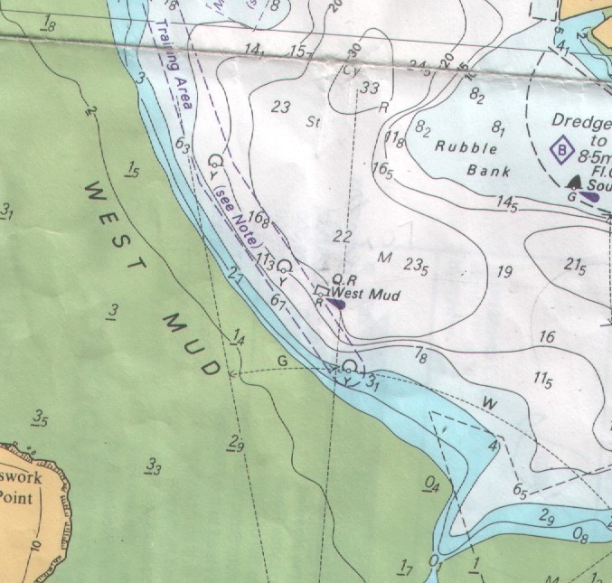
Figure 12 - Chart showing Locations of ADCP.	Figure 13 - Chart showing location of CTD dip at West Mud Buoy.

    The transmittance at all four CTD casts remains relatively uniform throughout the water column.  The only difference is in the relative amounts where there’s higher transmittance near site 10 due to deeper water and less turbulent mixing.

    Sites 5 and 6 showed marked increases in fluorescence at depths of 2 metres and 4 metres respectively.  Conversely, site 10 showed the same increase, however, it occurred at a depth of 8 to 10 metres due to reduced light attenuation.

    As CTD measurements were taken, the secchi disk depth was recorded. 

 

2.3.3 Nutrients       Silicate, nitrate and phosphate concentrations (µmol/l) were measured from water samples taken from the rosette bottles, during the deployment of the CTD. All three nutrients were plotted against salinity in order to obtain a mixing diagram and a theoretical dilution line (TDL) for identifying either conservative or non-conservative behaviour. Movement away from the TDL indicates non-conservative behaviour, whereas data points that fit this line show conservative behaviour.     Silicate-             The silicate mixing diagram, (Figure 14) illustrates silicate concentration change between the riverine and marine end members.  The mixing diagram suggests that the behaviour of Silicate in the Tamar Estuary is non-conservative, with greatest removal occurring in the upper reaches of the estuary, to the north of the River Tavy.  This pattern is likely to be the result of an increase in diatom abundance and the extraction of Silicate from the water column for the synthesis of their tests. 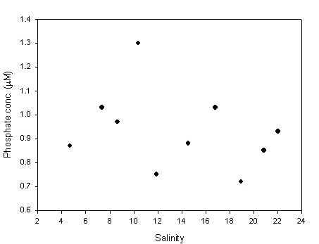This is supported by phytoplankton counts (chla_and_phytoplanktoncounts.xls) showing diatoms dominate the phytoplankton community.        Slight addition of silicate appears to occur in certain areas of higher salinity this could possibly be due to the weathering of rocks (e.g. near Beggar Island in the River Lynher) or due to an abundance of desiccated benthic diatoms across the mudflat (West Mud), washed into the Tamar as a result of eddying caused by the forcing of water round the dock walls. This physical process was identified in the ADCP data (Figure 2). Phosphate-               Phosphate decreases with an increase in salinity. Figure 16 illustrates that phosphate displays non-conservative behaviour throughout the estuary transect. However, between salinities of 0-20 there is significant removal of phosphate, whereas between 20 and 35 there is a clear addition of silicate. These behaviours might be explained by biological depletion of phosphate by phytoplankton populations, and the anthropogenic addition from the built-up areas of the lower estuary.  Nitrate-        Nitrate concentrations show a continuous non-conservative profile throughout the upper and lower estuary (Figure 15). This is due, again, to removal of nitrates from the water column by phytoplankton activity. There is no evidence for any anthropogenic addition similar to that found in the phosphate profile.
	Figure 14 - Silicate against salinity showing TDL.
	Figure 15 - Nitrate against salinity showing TDL.

Figure 16 - Phosphate against salinity showing TDL.	Figure 17 - Dissolved oxygen against salinity.

2.3.4 Dissolved oxygen 

    Water was collected from the CTD casts in order to measure dissolved oxygen using the Winkler method, and a value for oxygen concentration (µmol/l) was calculated. Oxygen concentration was plotted against salinity (Figure 17) to reveal any pattern between the riverine and marine end-members. The overall trend is an increase in oxygen concentration with increasing salinity. This general trend is explained by lower summer water temperatures in the marine compared to fresh waters, leading to a higher dissolution capacity in oceanic waters. The potential increased summer productivity of marine phytoplankton populations, which is supported by higher phytoplankton counts towards the marine end-member (chla_and_phytoplankton_counts.xls). 

2.3.5 Chlorophyll a and phytoplankton cell counts     Chlorophyll a (chl a) levels are plotted against salinity (Figure 18), because chlorophyll reflects nutrient levels which are, in turn, influenced by salinity.  This gives an indication of how chlorophyll concentrations vary between the riverine and oceanic end-members of the Tamar estuary. Overall, chlorophyll a (an indirect biochemical marker of primary production), decreases with increasing salinity, suggesting higher primary production near the riverine end-member.  This is possibly due to the high nutrient input from terrestrial sources, particularly during this period of relatively high rainfall and river discharge. High phytoplankton cell counts (chla_and_phytoplankton_counts.xls) are observed at salinities below 25, but high counts above salinities of 35 are also noted.     Nutrient plots against salinity suggest biological removal of silica, phosphate and nitrate towards higher salinities (with some possible anthropogenic input of phosphates at such salinities) which in turn suggests higher phytoplankton production. However the phytoplankton cell count patterns do not strongly reflect the biological uptake of nutrients, since they show high counts at both end members, as opposed to decreasing chlorophyll levels towards the sea. But considering the biology of phytoplankton, this loss of nutrients towards higher salinities is most probably due to such organisms.     Diatoms appear to be the dominant species, which might account for overall biological silica removal towards high salinities. However the pattern of diatom distribution, (similar to total phytoplankton cell counts): high near the riverine end-member, high at the oceanic end-member and low at intermediate salinities, does not clearly reflect the plot of silica against salinity (Figure 14).
	Figure 18 - Chlorophyll a against salinity

 

2.3.5 Zooplankton

    Horizontal trawls (200um mesh net) were taken for zooplankton samples at stations 6 and 11, to complement samples taken further up the estuary by rib. Analysis of samples by another group was not carried out, and so data was not made available for interpretation. It might be expected, however, that as general statements

a)      zooplankton abundance might increase towards the mouth of the estuary

b)      Both meso- and holozooplankton diversity will increase towards the mouth of the estuary.

c)      The dominance of the zooplankton community by particular groups, particularly hyperbenthic species, will increase higher up the estuary.

 

2.4 Summary

    The physical profiles made of the water column (with ADCP and CTD) revealed various processes: a flood tide entering the river Tamar via a northward flow, with the denser seawater moving below the lighter freshwater (presence of salt wedge), as well as strong thermocline and halocline at 5 m depth up the River Lynher, which decrease in strength and depth moving out towards Plymouth Sound due to turbulence and mixing.

Overall biological removal of silicate, phosphate and nitrate is apparent towards the marine end-member however this is neither reflected by chl a levels nor strongly  backed up by phytoplankton counts, although a dominance of diatoms may explain silicate concentrations. There is evidence of anthropogenic input of phosphates between 20 and 35 psu.

Dissolved oxygen levels are higher towards the marine-end member suggesting high phytoplankton production, this is supported by high phytoplankton counts at higher salinities. High dissolved oxygen levels could also be put down to lower marine water temperatures.

2.5 References

Uncles, R.J., Lewis, R.E, 2001, The transport of freshwater from river to coastal zone through a temperate estuary, Journal of Sea Research, p.173.

G.R. Tattersall, A.J. Elliott and N.M. Lynn, 2004, Suspended sediment concentrations in the Tamar Estuary, www.sciencedirect.com
Back to Top
 

 

 

---

Offshore Sampling (Terschelling)
3.1 Introduction 3.2 Position Data 3.3 Physical Analysis 3.4 Biological Analysis 3.5 Chemical Analysis 3.6 Conclusion 3.7 References   Back to Top
		R.V Terschelling

3.1 Introduction

       Results are presented from a survey of coastal estuarine water from the lower Tamar estuary. Previous studies in the area around Plymouth breakwater and Cawsand bay have revealed the presence of a freshwater mass in the area.  Biological chemical and physical techniques were used with the aim of determining the source and nature of the water body found. The main instruments used were a CTD, ADCP and plankton nets. A Secchi disk was also used to confirm the depth of the euphotic zone.

                                                                                                             Chart 2 - Sampling stations for Terschelling.

3.2 Position Data
     3.2.1 Tidal Information
      3.2.2 Position and Deployment Data

3.3 Physical Analysis

3.3.1 CTD Data  

  

From CTD and ADCP analysis a series of deductions are possible about the water of Plymouth Sound. The riverine water rounds the eastern coast of Drakes Island and enters Plymouth sound. Due to the shallow topography the area acts as an effective “mixing bowl”.  This is due to surface wind and wave action overlapping with bottom mixing by currents. This results in a well mixed water body, which is illustrated by data for station 9, (Figure 22), which shows uniform temperature and salinity readings of 14.6 ˚C and 34.363 respectively throughout the water column. This is further backed up by the Richardson number of 1.85, showing instability in the water column due to the low flow rates resulting in limited energy being needed to stratify the water column.  Station 1, taken off the western edge of the breakwater (Chart 2)  3 hrs before low water also shows a well mixed water column with a Richardson number of 3.11. At station 1 the water temperature had dropped by 1˚C relative to station 9 while the salinity has increased to 34.89. Salinity will have increased because the water body is further offshore, dispersing the freshwater influence of the River Tamar.

    A band of freshwater was found to be flowing South along the western edge of Cawsand bay which is illustrated by data from station 5 (Figure 20).  The layer of freshwater is at a depth of 2m, where there is reduction in salinity and an increase in temperature. The more saline seawater layer can be seen below the thermocline at 5.5m, establishing a stratified water body, with a Richardson number of 7.81.  The thermocline and halocline are initially separate but by station 7 they have been combined by the forcing of the lower seawater as it’s channelling between the breakwater and the land.

 

Figure 19 - Temperature Salinity Profile of Station 1	Figure 20 - Temperature Salinity Profile of Station 5

    As water bends around the headland at Penlee Point (50 19 153N 4 11 202W) it meets the denser seawater and is pushed up and over it, forming a thermohalocline which is pushed into the Sound with the flood tide, as seen at station 7 (Figure 21). This pattern is inherently very stable, with a Richardson value of 34.88 and virtually no mixing taking place. As the water moves into the Sound, the shallower depths, cause the surface mixing to coincide with the bottom mixing to again create a well mixed water column. (While averaging the data a problem was encountered with FSI Post, thus the top metres have been cut out of the profiles.)

Figure 21 - Temperature Salinity Profile of Station 7	Figure 22 - Temperature Salinity Profile of Station 9

3.4 Biological Analysis       3.4.1 Zooplankton community structure     Table 4 shows the results of zooplankton identification from the bottle samples. Vertical net samples were taken at depths dependent on the back scatter shown on the ADCP (chlorophyll maxima) and the structural data identified by the CTD. Station 2 shows that there is greater diversity and abundance of zooplankton at depth compared to the surface layer. By contrast at station 3 there is similar total abundance in both upper and lower samples. There is, however, a change in species type. The lower sample was taken within the thermocline and demonstrated a large abundance of gastropods compared to 0 in the upper sample.     The thermocline at station 4 was present at a depth of 6m and there was a greater abundance of zooplankton (6088 individuals per m3) above the thermocline compared to the sample taken below and through the thermocline (1796 individuals per m3). It was also clear that different species were present at the different depths with reference to the physical structure of the water column.     Again at station 5 the size of the populations in the surface 4 metres was greater than 4-8 metres. The surface layer was dominated by Noctiluca sp. Although the depth sample had fewer individuals there was greater diversity. The CTD profile of station 5 has shown the surface 4 metres of water to be fresher and warmer than the water the lower sample was taken in. It is clear that different species groups occupy different biological niches above and below the thermocline.
	Figure 23 - Decapod larvae
	Figure 24 - Copepod, Polycheate, Hydromedusae.
	Figure 25 - Decapod

3.5 Chemical Analysis
       3.5.1 Oxygen
       3.5.3 Nutrients
       3.5.4 Chlorophyll a

3.5.1 Dissolved Oxygen  

Dissolved oxygen data showed no consistent pattern when plotted against salinity. When plotted against depth the general trend within the data was a decrease in oxygen concentration with depth. Station 5 illustrates the typical dissolved oxygen profile found. This trend can be explained by surface wave activity increasing dissolved oxygen content at the surface and by zooplankton using dissolved oxygen for respiration at the surface of the water column. Large populations of zooplankton are not found in areas where there are low levels of dissolved oxygen. The rough sea on the day of survey is therefore the most likely cause of high dissolved oxygen levels in the surface 3 meters of water.

3.5.2 Nutrients           As the water masses surveyed were influenced by fresh water, nutrient concentration is plotted against salinity to produce horizontal mixing diagrams. Phosphate showed no consistent pattern when plotted against salinity and depth suggesting that for the sites investigated phosphate is well mixed horizontally and vertically. Silicate did show some variation in concentration (Figure 27). The concentration profile is non-conservative due to the removal of silicate. This removal is probably associated with the action of diatoms, which use silica to synthesise their skeletal tests. There is little vertical stratification for silica except at station 3, where most removal occurs at a depth of 10m (Figure 28). This removal is probably due to diatom growth at depth, where the maximum extent of the euphotic zone is at its deepest being 6 metres (Table 4).      Nitrate shows non-conservative behaviour with some addition to the water column further out to sea (Figure 26). Fresh water run off in the area is the most likely source of this nitrate.

Figure 26 - Nitrate TDL

Figure 27 - Silicate Theoretical Dilution Line	Figure 28 - Silicate profile at station 3

 

3.5.3 Chlorophyll a

 

Figure 29 - Profiles of chlorophyll at station 1	Figure 30 - Profiles at station 5

3.6 Conclusion

    The physical data identified a well mixed area located in Plymouth Sound and more stratification further out to sea. As the tide floods into the Plymouth Sound there is some superimposition of this off shore stratification. A layer of fresh water was also identified in the water column.

 

    Zooplankton data showed that different species occupy different biological nieces above and below the thermocline.

    Dissolved oxygen results showed a decrease in levels with depth as a result of wave action.

    Nitrate data shows addition offshore due to freshwater inputs and silica shows removal due to diatoms.

    The chlorophyll results for station 1 are atypical a decrease in chlorophyll levels down to 6 m but by 13m the levels returned to surface concentrations. Station 5 however did show a typical chlorophyll profile.

3.7 References
Morris, A.W., Howland, R.J.M., Woodward, E.M.S, Bale A.J., and Mantoura, R.F.C, 2003, Nitrite and ammonia in the Tamar estuary, www.sciencedirect.com 

 
Holligan, P.M, Williams, P.M, Purdie, D., and Harris, R.P, 1984, Photosynthesis, respiration and nitrogen supply of plankton populations in stratified, frontal and tidally mixed shelf waters, Marine Ecology Progress Series.  

Back to Top

 

 

 

---

 

Small Boat Work (Upper Estuary)
4.1 Introduction 4.2 Position and Sampling Data 4.3 Analysis
	R.V Ocean Adventure

4.1 Introduction
    The focus of the RIB survey was the biology of the upper reaches of the river Tamar; collecting zooplankton, phytoplankton, chlorophyll a and nutrients, as well as dissolved oxygen, salinity, temperature and depth readings. Samples were aimed to be taken at a fixed salinity interval of 2, and depth profiles were planned, to obtain an idea of the physical structure of the water column. Unfortunately, the survey was cut short due to technical failures on both RIBs, we shall therefore present the data obtained between 4 and 22.

 

4.2 Position Data

      4.2.1 Tidal Information

      4.2.2 Position and Sampling Data

 

4.3 Analysis

4.3.1 Nutrients  Nitrates        On the plot of nitrate concentration against salinity (Figure 31) a theoretical dilution line (TDL) was drawn. We observe an overall decrease of the nitrate towards higher salinities. The data is distributed along the TDL revealing a conservative mixing pattern for nitrates, which suggests no net biological removal (although biological removal may occur, the inputs may balance it out). Phosphates        The plot of phosphate concentration against salinity (Figure 32) shows a slight increase in concentration with increasing salinities, and clear non-conservative behaviour (data points diverge from the TDL) in no particular pattern of addition or removal. This apparent lack of clear pattern could be due to sporadic anthropogenic inputs of phosphates from the surrounding agricultural land on the banks of the Tamar.

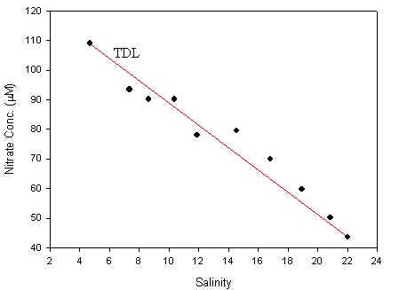Figure 31 - Nitrate vs Salinity showing the TDL.

Silicates 
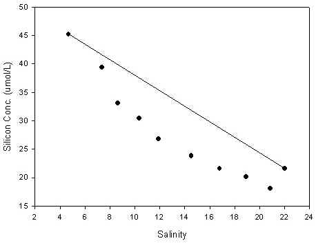
       Silicate concentration clearly decreases with increasing salinity and displays non-conservative mixing (Figure 33). There is clear removal of silicate which could be linked to diatom populations developing, and less anthropogenic addition of silicates which would potentially balance this biological removal out.  

Figure 32 - Phosphate against salinity.	Figure 33 - Silicate vs Salinity showing the TDL.

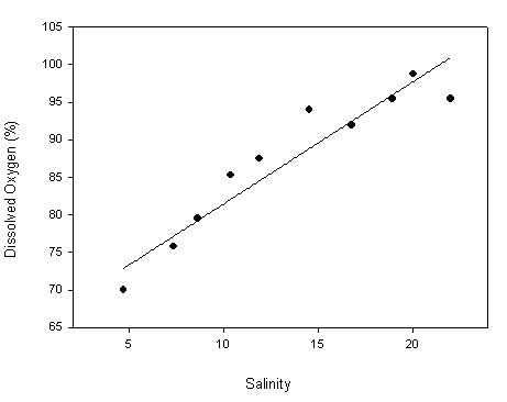
4.3.2 Dissolved Oxygen

       Generally dissolved oxygen increases with salinity (Figure 34), this could be down to the influence of colder oceanic waters which have a higher dissolution capacity compared to the warmer fresh waters, and possibly also due to increased activity of marine phytoplankton which develop towards higher salinities, but as this is not reflected in the chlorophyll a data, it is likely the dissolved oxygen pattern is linked to physical processes rather than biological ones. 

 

Figure 34 - Dissolved oxygen against salinity.	Figure 35 - Chlorophyll a against salinity.

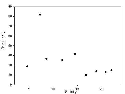
4.3.3 Chlorophyll a
       The overall trend is a decrease in chlorophyll a (chl a) with increasing salinities, which suggests that there is a strong development of phytoplankton species which are better adapted to less saline waters and hence different from marine species which would develop in much stronger salinities > 30, it is therefore possible that chlorophyll levels increase towards stronger salinities, however we have no data available to draw any such conclusions (Figure 5).   

 

4.3.4 Zooplankton

       Unfortunately, zooplankton samples were unable to be collected and analysed for the area covered by the small boat work. This was due to failures with both boats, resulting in termination of the sampling.

 

 

 

 

 

 

 

---

 

Appendix

• Appendix 1 Geophysical Survey

• Appendix 2 Lower estuary sampling (Bill Conway)

• Appendix 3 Offshore sampling (Terschelling)

• Appendix 4 (Small Boats)

 

---

Appendix 1 Geophysical Survey (Nat West II)

 

1.2.1 Tidal Information

    26/06/04 - High Water - 11:22 GMT    Low Water - 17:33 GMT      Neap tides

 

1.2.2 Transect Data

 

Area	Transect	Position Started	Position Finished	Notes
Bridge	1	50º 24.54 N  04º 12.21 W	50º 24.13 N 04º 12.22W
Docks	2	50º 23.49 N 04º 12.48 W	50º 23.31 N 03º 11.98 W

 

Back to Geophysics

---

Appendix 2 Lower estuary sampling (Bill Conway)

 

2.2.1 Tidal Information
   29/06/04 - High Water -  14:42 GMT     Low Water - 08:32    3 days after neaps tides.

 

Back to Lower Estuary Analysis