Jo, Charlotte, Alex, Tom, Oli, Jenny, Helen, Rachel and Sarah
| Abstract |
| Introduction |
| Geofield |
| Estuarine Environment |
| Offshore Environment |
| Coastal Environment |
| Geophysics |
| Conclusion |
| References |
The main aim
of this practical exercise was to gain a holistic view of the River Tamar
estuary and adjacent coastal region, and study the associated processes. The
sampling and surveying ranged from the head of the salt water intrusion (a
salinity of 0.16) to the E1
monitoring point (50.02.070N 4.52.535W), approximately 25 kilometres offshore. A
variety of sampling and data collection methods were utilised, notably CTD, ADCP,
T-S probes, Side-Scan Sonar, plankton nets and nutrient sampling. The data was
then analysed to produce a complete picture of the entire estuary.
The
survey of the upper estuary showed evidence of a salt wedge during the incoming
tide, as well as temperature profile, with a change of 0.5°C
from the warmer riverine water to the cooler estuarine waters. The nutrients
showed very different results: Silicate showed non-conservative behaviour, with
removal in the upper estuary probably due to uptake by diatoms. Phosphate also
showed non-conservative behaviour, with both addition and removal associated
with areas of past and present industrial use. Nitrate showed slight addition in
the upper estuary, with slight removal in the lower estuary due to uptake by
plankton as well as de-nitrification which reaches a maximum during summer. The
plankton data showed an inverse relationship between the zooplankton and
phytoplankton due to grazing. There is a difference in species dominance
throughout the estuary. Diatoms show dominance in the upper estuary, with 75% of
the total abundance, where Dinoflagellates dominate in the lower estuary, with
90% of the total abundance. Copepods tend to be the dominant zooplankton species
throughout the entire estuary.
The
offshore survey showed a phytoplankton bloom extending from the mouth of the
estuary, offshore to a water depth of 50 meters, as well as various other areas
of backscatter indicating plankton maxima at depth. At the E1 monitoring station
we recorded a very distinct thermocline at a depth of 29 meters, with
fluorescence maxima (4.0 micrograms per litre) at 28 meters. This fluorescence
maxima coincided with a backscatter peak from the ADCP data indicating
zooplankton grazing. The fluoresence maxima occurs just above the thermocline
because nutrients leach slowly through it, enabling the phytoplankton to take
advantage of the available nutrients. In the zooplankton net that was taken in a
vertical plane through this backscatter peak a huge abundance of large
unidentified cnidarian plankton was found, which were approximately 2cm in
diameter. Backscatter peaks were also identified above the two peaks of
Eddystone Rocks which were covered; this coincided with a decrease in the depth
of the chlorophyll maxima which was noted on the miniBAT transect in the same
area.
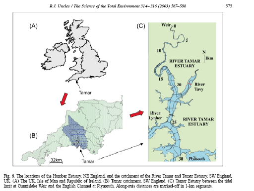
The major freshwater inputs to the Tamar estuary are the Rivers Tamar, and the Tavy and Lyner which are sub estuaries which junction with the Tamar. The yearly averaged runoff from the River Tamar based on runoff records for 1976-1990 is 22 m³s‾¹ and the Tavy and Lyner contribute and additional 27 and 23% of the Tamar’s flows respectively (Uncles et el 2001).
Tides in the Tamar estuary are semidiurnal, with mean neap and spring ranges of 2.2 and 4.7m respectively. The Intra-tidal variations in total water depth are therefore considerable in the shallow, upper reaches (Uncles et al 2001).The water transport on the flood tides separates at the junction of the Lyner and Tamar in the ratio of approximately 30 and 70% respectively. This ration is approximately the same for the junction of the Tavy and Tamar (Uncles et al 2001).
During the summer months, the inshore waters of Plymouth Sound, tend to be dominated by a halocline. However, further offshore, thermal stratification starts to dominate. Current speeds are strongly influenced by the bathymetry of the Sound and subsequently in combination with wave action influence the distribution of bottom sediments. Fluvial input is relatively small and it is suggested that coastally derived sediment brought into the sound during severe storms, locally eroded material and a small yet important anthropogenic input in the form of eroded material from the breakwater and ship ballast, make up the bottom sediments (Allen et al 2003).
The geology around
Aims
The
Aims of this field trip are relatively straight forward,
|
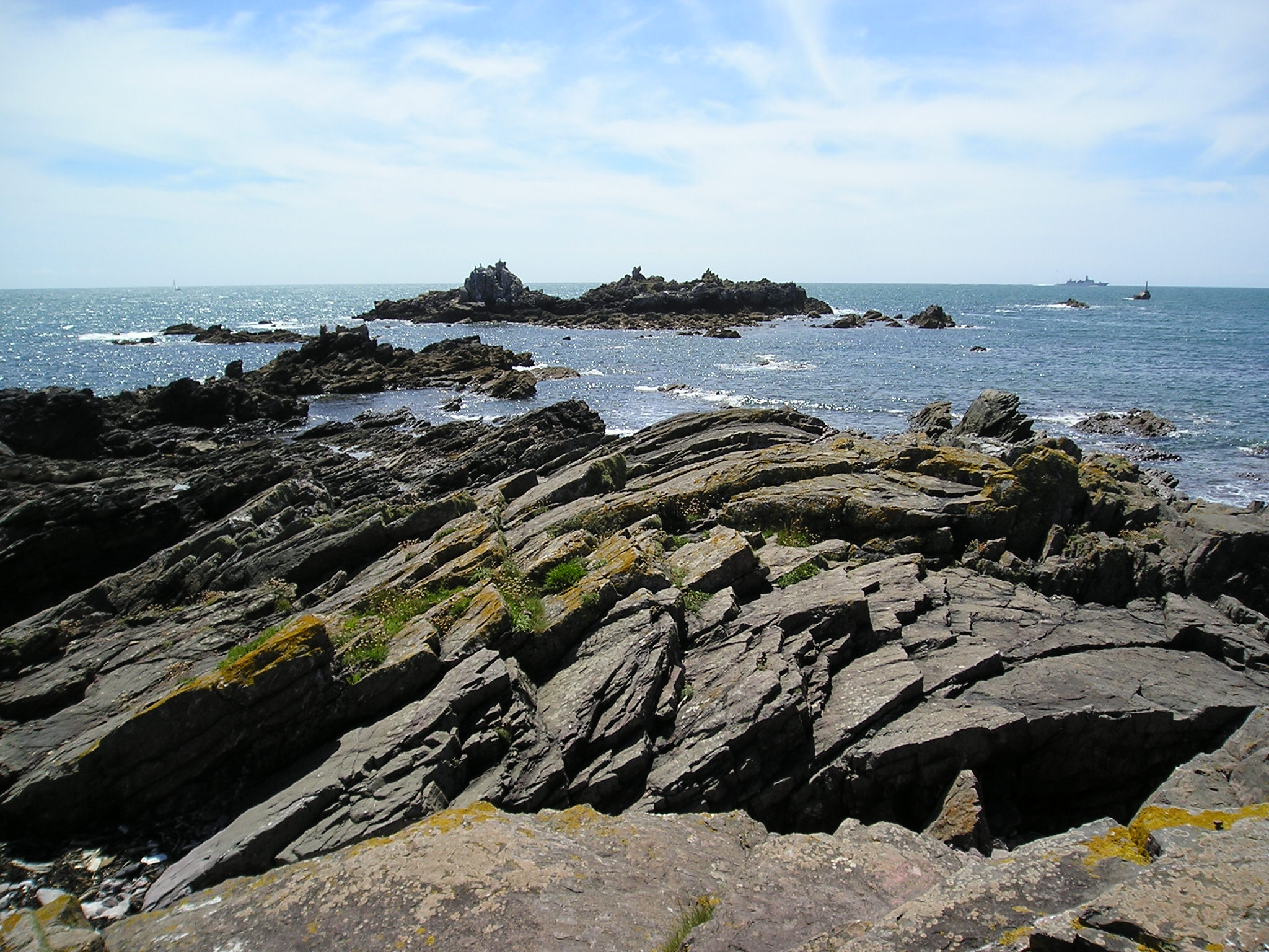 |
Introduction The investigation was carried out on Friday 25th June 2004.We visited a rock exposure at Heybrook Head known as Renney Point on the shoreline of the eastern coastline of Plymouth Sound. The precise location of the exposure is illustrated below: |

(Click to Enlarge) |
|
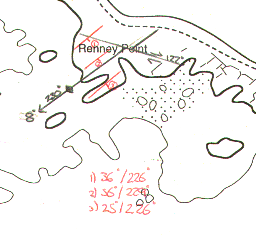
| Fig. 2 - Ordnance Survey map of the survey area | |
| Fig. 1 - Image looking down the axial trace of the antiform, the fold being indicted by the curvature of the rock units. |
|
Aims
Methods
Results At Renney Point initial investigation was to take a dip and strike of some of the rocks exposed on the shore. This was mainly used as an instructional section as to how to use the compass clinometer. Initially a strike of 226º and a dip of 36º were found, another set of measurements were conducted approximately 30 meters to the southwest of the first point and a strike of 226º and a dip of 25º were found. In between these two sets of measurements there was one very noticeable geological structure - an antiform fold. The axial trace of the fold was orientated to 230º and was plunging to an angle of 8º in the same direction. However, further up the beach the fold stopped at a trench within the rocks. This was a fault line that ran through the entire section of the rocks. The fault was a right lateral fault, otherwise known as a right dextral fault. The fault was orientated to 118º and had an approximate displacement of 5 meters. These results are shown on the geological plan. (shown in fig 4): |
 |
||||||||||||||
| Fig. 3 - Image of axial trace of the fold | |||||||||||||||
 |
|||||||||||||||
| Fig. 4 - Geological plan of Renney Point | |||||||||||||||
 |
|||||||||||||||
| Fig. 5 - Right dextral fault |
  |
Within the main fold that was studied a series of stress fractures were found. These all appeared to be orientated in similar directions. The orientation angles varied between the two maxima of 80º and 160º. This common direction of fracture is due to the direction from which the rock unit was forced in the past. In order for the fold to have a strike of 230º, the stress must have been applied in the 140 to 320º approximate direction. This would suggest that the fractures of the higher angles occurred first. It would also suggest that following this period of stress, the angle from which the stress was applied changed, thus producing the fractures at the lower angles. This statement can be reinforced by applying the law of cross cutting relationships. Two intersecting stress fractures were found. The law of cross cutting relationships states that when one rock fracture cross cuts another, the one that does the cross cutting is the younger. In the field a 147º fracture was intersected, and slightly displaced by the fracture at 97º. This shows that the the angle of stress applied to the fold changed over time. |
|
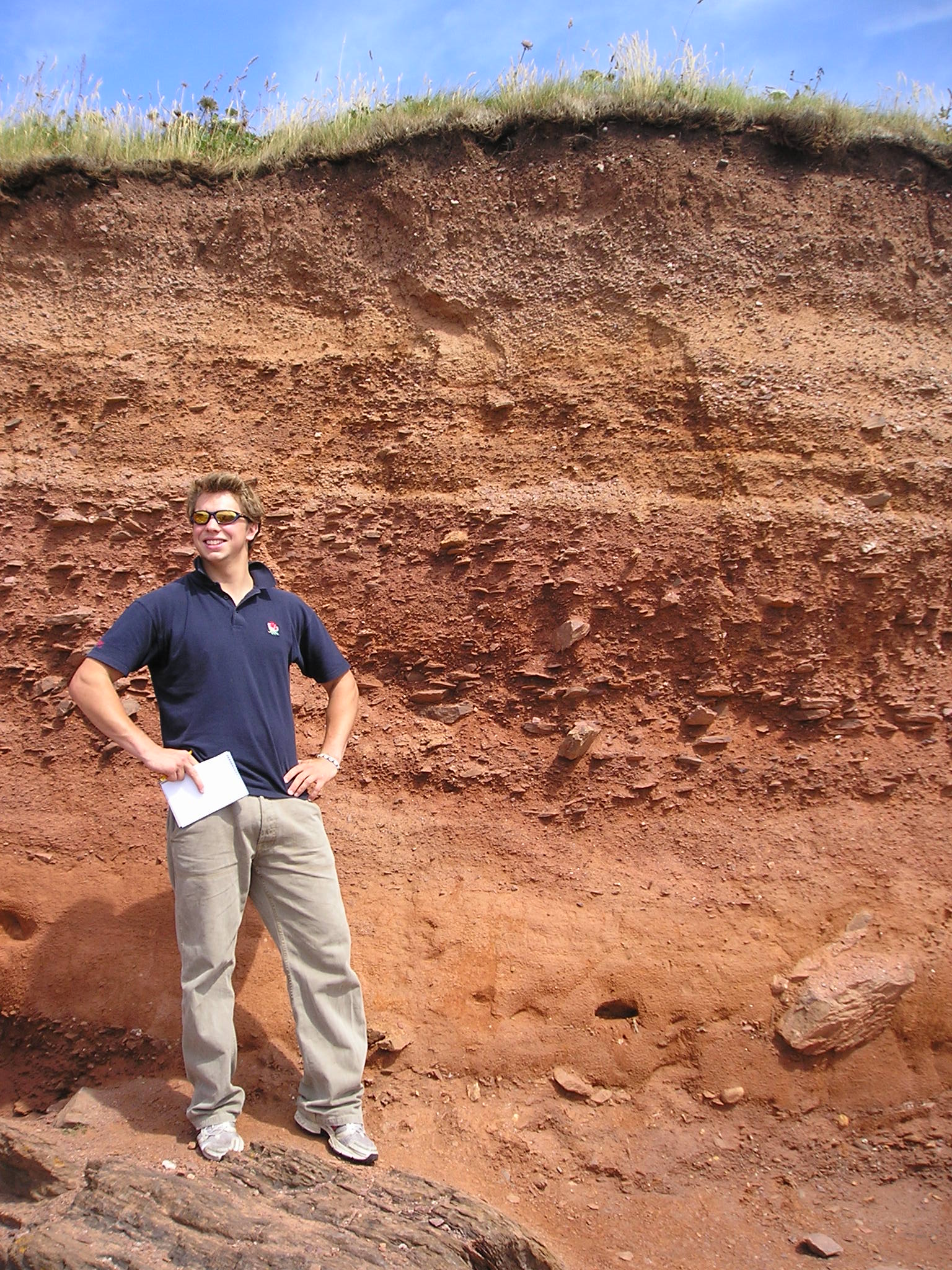
| Fig. 6 - Illustration of the sediment exposure | Fig. 7 - Image of the sediment exposure with person to scale | |
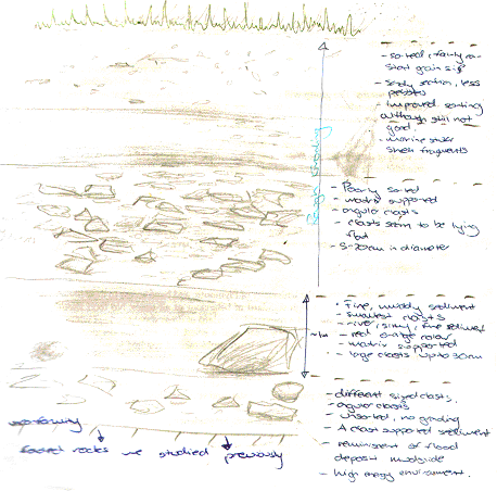
Once the hard rock geology was analysed, a survey was completed of the sediment overlying the rocks. It was deposited from a periglacial environment during the latest period of glacial advance. This was the Pleistocene period which was at its maximum extent 18000 years before present. The sediment face was sketched and detailed observations were made. These are shown on the illustration below of the sediment exposure (Fig. 6) which was approximately 3.5 meters from top to bottom.

|
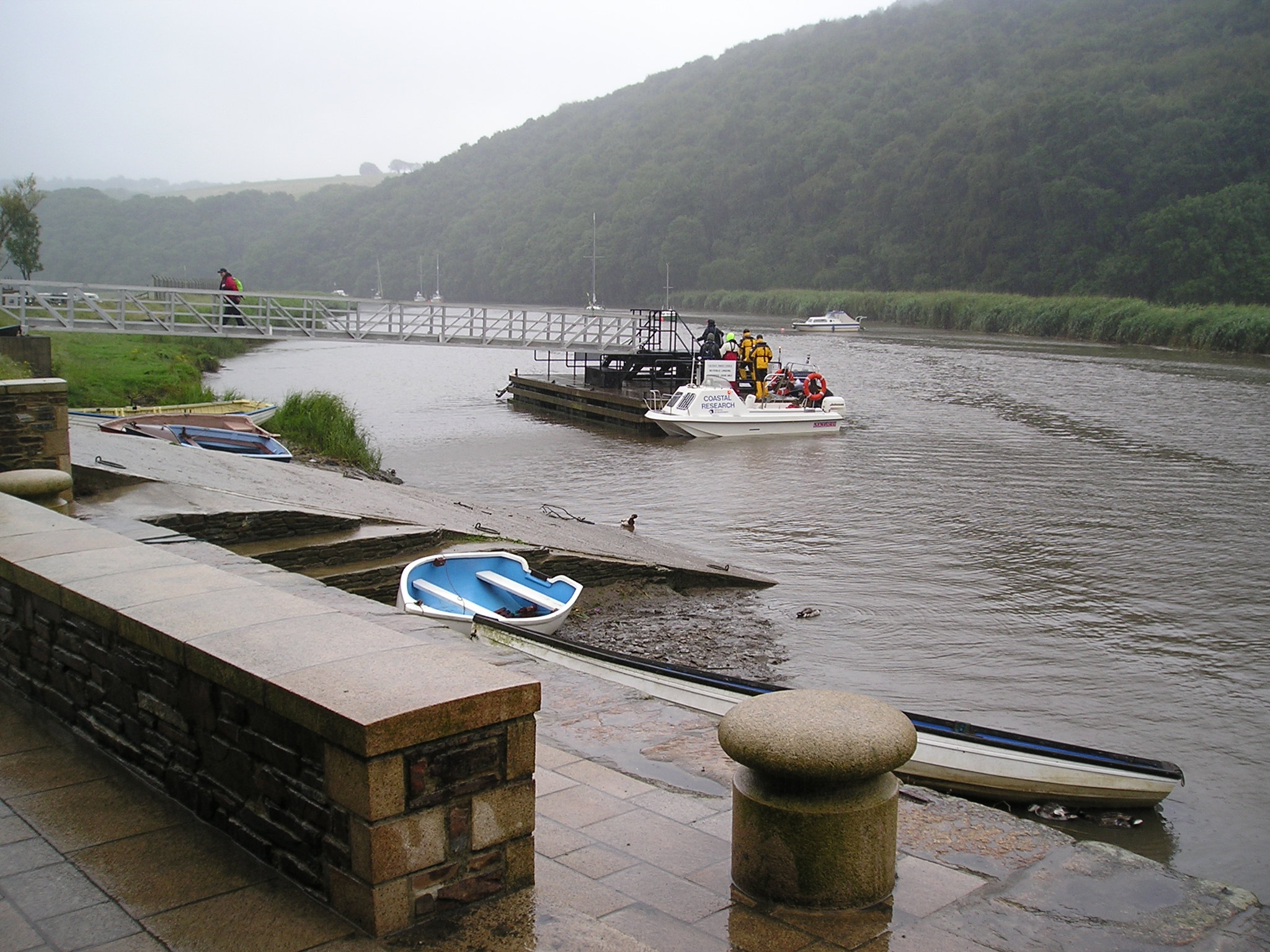
Introduction The investigation was conducted on the 26th June 2004, the weather in the morning was persistent rain, overcast, with 8/8 cloud cover. The afternoon brought intermittent showers, persistent drizzle with very low cloud cover (8/8). The winds were varying from 0 m/s to 7m/s with a direction ranging from 110° to 190°.Two RIBS were used to cover this 21 kilometre stretch to allow access to the upper reaches of the river. High tide (on the neap cycle) was at 11:22 GMT and therefore it was decided to travel to the furthest point upstream at the start and return towards Plymouth sampling on the way. |
|||||||||||||||||||||
 |
Aims
Methods
|
||||||||||||||||||||
| Fig. 8 - Image of the riverine end member of the Tamar estuary | |||||||||||||||||||||
 |
|||||||||||||||||||||
|
Fig. 9 - Tamar estuary location and catchment |
|||||||||||||||||||||
|
Results Salinity Section and Temperature SectionA salinity section was constructed for the length of the Tamar estuary. The vertical profile data obtained at each salinity value, with the multi parameter water quality monitor, was used to show the changes of salinity with depth. With reference to Fig. 10, there is vertical variation in salinity along the entire length of the twenty two kilometre section of the Tamar studied. This is more exaggerated in the upper reaches with a notable salt wedge at the lowest salinities of 0 to 8. Despite the presence of the salt wedge in the upper reaches, the rest of the estuary appeared well mixed. In areas with a faster water flow, there is an increased level of turbulence with the bed and banks of the river, which gives rise to higher levels of mixing. This is shown at the change between the salinities of 10 and 12, as well as 16 to 18, where the surface distance between the values is approximately 0.5km. The further down the estuary, into the deeper waters, the salinity changes become more spatially distant. This is exemplified by the salinity change of 28 to 30, where the distance between the two values appearing at the surface was approximately 3km. The overall temperature change through the section is less than one degree. The temperature section shows the warmer less saline water remaining on the surface as one moves downstream with salinity, and the cooler more saline waters beneath. |
(Click to Enlarge) |
|
Fig. 10 - Salinity Section |
|
(Click to Enlarge) |
|
|
Fig. 11 - Temperature Section |
|
Nutrients The factors affecting non conservative behaviour of nutrients can be broken down into biological removal/addition processes and non biological processes. Silicate - The silicate curve does not keep to the Theoretical Dilution Line, this is caused by removal in the upper reaches of the estuary followed by relative conservative behaviour towards the mouth. The removal in the upper estuary could be caused by a number reasons for this removal occurring. Diatoms are the most likely of the biological possibilities. Diatoms extract Silicate from water in order to create Silicate based frustules. This removal is often of the degree to cause a noticeable “dip” of this kind. There is a large increase in the relative abundance of Diatoms in the lower salinity region. This rise in Diatom numbers coincides with the removal of Silicate already observed. There are other possible causes for this decrease in concentration, one of which is the presence of two tributaries at the salinity regions of 8 and 10, which also coincide with the “dip”. The reason for an observed removal could be dilution by non silicate rich waters. However this dilution would probably not be to a significant enough degree to warrant the amount of removal seen, and would be likely to lower the salinity further if it was significantly influential. Phosphate - The phosphate curve exhibits non-conservative behaviour with both addition and removal with a rather “meandering” movement between the two. In the upper reaches, there is addition of phosphate to the water, however this changes to removal in the middle section of the estuary and returning to addition around the Tamar Bridge. The addition coincides with areas of past or present industrial land use, linking to sources of chemical pollution, such as fertilizer or sewage, and therefore human dwellings and their subsidiaries e.g. cattle, become sources of phosphate. These and other sources have been marked on the diagram where they occurred. At salinity region of two there is a single point of addition, this appears to be a large deviation from the TDL and corresponds with the presence of a sewage works in the near vicinity. Removal in the 8-12 salinity region is connected to the low density of houses and human features here than the rest of the estuary, in lower salinity regions of up to a salinity of approximately ten, flocculation is an active process that must be considered. A single point case of addition is seen at 14 salinity and could be because of the presence of a freshwater river that may have a particularly high phosphate concentration. After this point the “meandering” of the curve becomes less severe with only small changes to the rate of dilution of phosphate corresponding to small changes in the degree of human dwellings or their subsidiaries. The next area of non-conservative behaviour begins at a salinity of ~27 and carries on until the 33-34 region. It seems that the high degree of human/machine waste entering the water from Plymouth accounts for a large amount of phosphate entering the water column. The deviation from the TDL in this area is not as large as the upstream case of addition but there is a nine point deviation suggesting a high volume discharge, which would coincide with Plymouth being downstream. The time at which the samples were collected is an important factor, as they were taken just after high water when the tide was ebbing. Nitrate - The nitrate estuarine mixing diagram shows a slight addition to the upper estuary (salinity 4-8) and an equally small removal of nitrate at higher salinities (20-30). There are three main processes that can be responsible for modifying the nitrate concentration; nitrification, denitrification and biological uptake. The main sources of nitrate are related to the leaching of soil and surface runoff. The increased use of inorganic fertilisers and the anthropogenic NH4+ from car exhausts are the main reasons responsible for this increase. The decrease of dissolved nitrate (20µmol l-1) shown in the lower reaches is not only due to the uptake of nutrients during plankton growth but also due to denitrification, which is at a maximum during summer. The oxygen data was
considered to be inaccurate due to errors in the probe readings. It is possible
that olive oil spilt on the rib deck caused the TS probe to take inaccurate
readings.
|
|
(Click to Enlarge) |
|
| Fig. 12 - Silicate Estuarine Mixing Diagram | |
(Click to Enlarge) |
|
| Fig. 13 - Phosphate Estuarine Mixing Diagram | |
(Click to Enlarge) |
|
| Fig. 14 - Nitrate
Estuarine Mixing Diagram |
|
Phytoplankton and Zooplankton Figure 15 gives an overall view of the phytoplankton and zooplankton population fluctuations from the head to the mouth of the estuary. There are very few data-points for the zooplankton, little can be assumed from these, but the general trend is an inverse relationship between the zoo- and phytoplankton (site some references), as the phytoplankton are kept down by the grazing of the zooplankton. However, the change in phytoplankton abundance is only slight, and subject to speculation. The slightly higher concentrations of phytoplankton upstream, may be due to higher nutrients further up the Tamar, from surface run-off. Zooplankton, however, are more concentrated towards the mouth. There are fewer freshwater species of zooplankton, explaining the small numbers in the sample, and even fewer resident riverine populations, as the conditions are extremely stressful with the fluctuating salinity. It has been suggested that the plankton found there are simply those left over from the previous tide and do not survive for very long. Also, as the sampling was only taken up to around a salinity of 9, the fresh water species are unlikely to have been sampled at all. Fig 16 shows clear trends in species dominance in different areas of the estuary, with a diatom maximum at the head, and a dinoflagellate maximum at the mouth. The thermal stratification diagram (Fig. 11) shows strong mixing at the head, with slight stratification further downstream. Due to this, phytoplankton populations in the mixed water are composed mainly of chain forming diatoms, which require less light than dinoflagellates . There is likely to be more suspended material higher up, where the surface run-off occurs, reducing the light penetration, and creating an environment more suitable for diatoms, which are kept up in the surface layers by tidal mixing (Holligan, P.M. et al 1984). Dinoflagellate populations were found mainly in the more stratified waters, further down the estuary, where there is sufficient light in the thermocline for the bloom (Holligan, P.M.et al 1984). Ciliate populations were reduced to nil in the area of the dinoflagellate bloom, as dinoflagellates may be competing with ciliates for pico- and nano-plankton, and heterotrophic species could even be grazing on them (Rodriguez, F. et al. 2000)(Pierce & Turner, 1994). Ciliate populations are also generally higher at head of estuary, which may be due to the fact that large ciliates are controlled by predation-principally by copepods which are found in large numbers towards the mouth (Rodriguez, F. et al. 2000) (Nielson & Kiorboe, 1991, 1994). But these are only speculations, as this is a complex food web, and without further identification of individuals down to species level, we cannot make too many assumptions. Fig. 17 shows fewer zooplankton individuals at the head, increasing towards the mouth of the estuary, with copepods as the dominant family. This is to be expected, as copepods usually dominate the marine mesozooplankton in respect to numbers and biomass in all marine waters (Miller, 2004). Variations in zooplankton populations are mainly controlled by hydrodynamics of water column and physical effects on phytoplankton. Some species maintain important populations deeper in the pelagic zone throughout winter, so are more likely to be found in the deeper waters downstream (Rodriguez, F. et al. 2000). There are also generally fewer species at the head, increasing towards mouth. This is due to the fact that there are more saline zooplankton species than freshwater species. The oceans are more dynamic, so there are a wider variety of habitats to adapt to over evolutionary time, thereby increasing the zooplankton gene pool, whereas the freshwater systems are generally more stable, and gene pools have been more restricted, resulting in fewer varieties of zooplankton.
|
(Click to Enlarge) |
|
Fig. 15 - Plankton Relationship Abundance graph |
|

(Click to Enlarge) |
|
|
Fig 16. - Phytoplankton Species Relative Abundance |
|
(Click to Enlarge) |
|
|
Fig. 17 - Zooplankton Species Relative Abundance |

Terschelling |
Introduction The Terschelling data was collected on the
29th of June 2004 between 0900 and 1700 GMT. Thermal stratification (especially during
the summer months) is very dominant in waters off The aim of this trip offshore was to
determine how vertical mixing processes in the waters off Plymouth affect,
directly and indirectly, the structure and functional properties of plankton
communities in the coastal waters of the western English Channel. |
|
Methods
|
Minibat |
||||||||||||||

CTD |
(Click to Enlarge) |
Results Minibat The
minibat data recorded on Tershelling was obtained by taking 2 transects from
station 2 at the E1 monitoring point(50.02.070N 4.52.535W), in the direction of
eddystone rocks. The transect started at 12:35 GMT and finished at 13:40 GMT
with a 10 minute interlude at 12:45 due to the minibat not diving below 14m. At
this point the fixed fins were adjusted (files E1tonorth and E1tonorth2). A
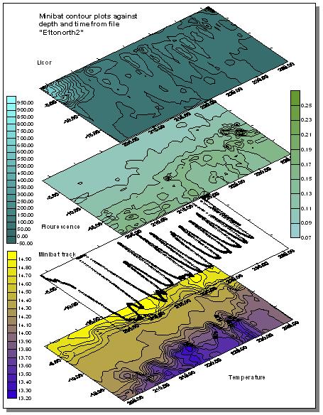
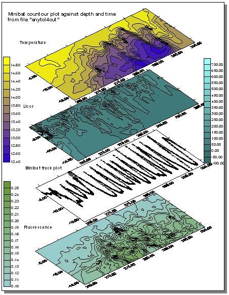
second minibat transect was taken from just before The
minibat generated data on celerity, conductivity, temperature, density,
fluorometry, oxygen, salinity, transmission and light attenuation. The data was
coverted into plots using the Surfer package. Plots of temperature, fluorometry,
light attenuation and minibat track against depth and time were created. Plots
of salinity and transmissometry were discarded due to the nature of the offshore
water we were sampling. The first minibat transect showed that there is a distinct thermocline and a stratified water column. The
second minibat transect from a random spot to L4 showed a fluorescence maximum
occurring. This was corresponded with an area of high backscatter on comparing
the ADCP data. This is indicative of the presence of phytoplankton, and
chlorophyll maximum in the water column. There is also evidence of the
thermocline being forced upwards in the water column. The location of this was
to be found in the area of |
| Fig. 18 - Minibat transect 1 maps | |
(Click to Enlarge) |
|
| Fig. 19 - Minibat transect 2 maps |
|
Acoustic
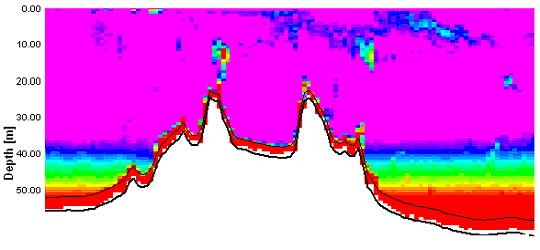
Doppler Current Profiler Data As one can
clearly see in figure 20, there is a tongue region of high backscatter that protrudes from
the mouth of the estuary. This shows that there is some suspended material
within the water column that is interfering with the beam of the ADCP. The next
step is to find the origin of that material: land derived suspended sediment, or
a plankton bloom, that is utilizing the nutrient rich estuarine waters, and
extending out into the more oceanic, nutrient depleted waters. To investigate
this it is necessary to study the CTD profile data for turbidity and fluorescence that
was found at station 1. This shows that the profile for fluorescence is
practically identical to that of the turbidity. This indicates that the water
column turbidity is almost entirely due to the suspended phytoplankton within
the water. Thus the high backscatter is indeed a planktonic bloom extending from
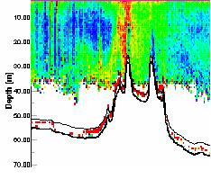
the nutrient rich estuarine waters, out into nutrient depleted, coastal waters. Figure 21 shows the ADCP backscatter data for our second sampling site, E1. As is clearly visible there is a region of higher backscatter at approximately 28 meters. It was suspected that this was a layer of dense zooplankton, so a plankton net was used to sample through this layer from 35 to 20 meters. This sample produced some very interesting results. It was calculated that for this particular trawl, a volume of 3.2m3 of water passed trough the net. Within the sample approximately 300 unidentified cnidarian plankton were found, of approximately 2cm diameter. It was likely that this plankton species was responsible for the strong backscatter of the emitted pulse. A similar scenario was observed at sample site 3 (see figure 22) at a depth of 10 to 13 meters. This final transect recorded data between sites 3 and 4, travelling northwards to the west ofTwo peaks
were found in backscatter above the shallowest sections of the A velocity peak around the
|
 |
| Fig. 20 - ADCP Section showing backscatter tongue | |
 |
|
| Fig. 21 - ACDP Section showing jellyfish backscatter | |
 |
|
| Fig. 22 - ADCP section showing shallow backscatter peaks | |
 |
|
| Fig. 23 - ADCP Section showing backscatter maxima |
(Click to Enlarge) |
CTD
Profiles The
first site sampled was site 1 within the estuary, just behind the
breakwater. The fluorescence shows a subsurface peak at approximately 7 meters. Thus, it is assumed that there is a phytoplankton maximum at that depth. The ADCP data reinforces this assumption, as a backscatter maximum was seen at the same depth. This
again is consistent with the high backscatter tongue that protruded from the
mouth of the estuary. The tongue is formed from the backscatter that reflects
off the zooplankton within the water column. This however, this will also be
where the phytoplankton are located. This assumption can be made due to the fact
that zooplankton graze upon phytoplankton, therefore they will generally occur
in the same location within the water column, despite the zooplankton being more
motile. The subsurface maxima at site 1 may help to explain the spatial
distribution of the bloom extending out of the estuary. Referring to the
ADCP data from figure 20 one can see the bloom extending offshore. It is
notable that the bloom disappears from the uppermost surface waters at
approximately 6 kilometres offshore, however, the bloom continues at a depth of
10 metres for another 6 kilometres, until it finally dissipates at 12 kilometres
offshore. The
nutrient analysis shows large reductions in the concentrations of both phosphate
and nitrate. Silicon concentrations are also lower at this depth the
concentration falls from over 2.5umol/l to 0.6umol/l. This removal is caused by
the uptake of silicon for the production of skeletal material in diatoms,
another indicator of a bloom. As it would be expected with a bloom of this type
there is a dramatic increase in oxygen concentration at depth and the
chlorophyll levels also increase. In
terms of the data collected by the on board instruments the presences of the
bloom observed form the nutrient data is corroborated. The CTD vertical profile
shows an increase in the fluorescence at a depth slightly deeper than, estimated
from the lab work, closer to 30m. The
data collected by the ADCP also indicates an area of high backscatter caused by
suspended organic matter (see figure 21) There is a very defined thermocline at an approximate depth of 29 metres. This may explain why there is a fluroesence, and henceforth, chlorophyll, maxima at a depth of 28 metres. If the ocean were fully mixed, it would be expect that the maximum phytoplankton growth were at the surface, where there is maximum light intensity. However, in this situation, the thermocline affects the location of the point of maximum phytoplankton growth. With a secchi depth of 10 metres, it would be expected that the depth of the euphotic zone (k) would be 30 metres ( k = 3 x secchi depth) Despite this, there is minimal growth above the thermocline due to a lack of nutrients. The chlorophyll maximum occurs just above the thermocline as nutrients are gradually leached through. Thus the plankton can utilise these leached nutrients and form a significant population.
|
| Fig. 24 - Temperature, Transmission and Fluorescence at Station 1 (breakwater) | |
(Click to Enlarge) |
|
| Fig. 25 - Temperature, Transmission and Fluorescence at Station E1 |
|
Phytoplankton Site 1 was near the breakwater, thus there were several dominant water streams in the locality. Mostly chain forming diatom species were found to be dominant with an overall decrease in phytoplankton abundance from surface to depth. This coincides with an increase from surface to depth in nitrate concentrations. L4 was the next site offshore but the 4th site visited. Again, chain forming diatom species were dominant with a similar decrease in abundance of phytoplankton with depth. Here the Secchi depth was10m, therefore 1% euphotic depth is approximately 30m bottom community (below 30m), causing the populations of phytoplankton to be light limited. Site 3 was in between Site 2 was the furthest sample site offshore at point E1. As with all previous sites, chain forming diatom species dominant but small clumps of Phyocystis began appearing in samples. The thermocline was found at 28m with the deep chlorophyll maximum present above the thermocline at 27m. This implies that the phytoplankton community above the thermocline was probably nutrient limited and the population below the thermocline probably light limited, but is located at the nutricline (where the maximum change in nutrient concentration occurs).
|
(Click to Enlarge) |
| Fig.26 - Phytoplankton abundance change with depth | |
(Click to Enlarge) |
|
| Fig.27 - Phytoplankton Abundance | |
(Click to Enlarge) |
|
| Fig. 28 - Relative Abundance of Phytoplankton | |
(Click to Enlarge) |
Zooplankton One aim for Terschelling was to see if there is a change to zooplankton abundance and community structure as you go further offshore. Fig. 29 shows that dinoflagellates (especially the
heterotrophic species Noctiluca) were
highly abundant, except at site 2 (E1) depths 56 – 35m, which according to the
Secchi disc depth of 10m would be below the 1% euphotic zone. Possible reasons
for why Noctiluca was not found in
this area could be caused by the physics of the water column. The presence of a
thermocline found at 29m may act as a barrier, stopping penetration of Noctiluca
below this depth. Noctiluca is a
heterotrophic dinoflagellate that feeds on small zooplankton (as well as on
diatoms and other phytoplankton) (Lalli & Parsons, 1997) and so will want to
be where the phytoplankton is located (i.e. in the euphotic zone).
At site 2 (E1) the deep chlorophyll maximum was seen on the upper edge of
the thermocline (at 28m), this should lead to a large presence of zooplankton
due to the high abundance of food.
|
| Fig.29 - Relative Zooplankton Abundance |
|
Table
1: the changing dominance of species with depth at site 2 (E1) |
||
|
depth |
Copepods
% abundance |
Dinoflagellates
% abundance |
|
surface |
0.8 |
97 |
|
35 –
20m |
18 |
70 |
|
56 –
35m |
85 |
1.8 |
The relative
abundance of copepods increases with depth at site E1, as the dominance of
dinoflagellates decrease shown in table 1. This major change in abundance occurs
over a dense layer of cnidaria and other jellies. Copepods feed by filtering
phytoplankton and protists from the water column or by carnivory,
(Miller, 2004). Small jellyfish are part of the
copepod diet and would supply a food source to
Copepods in waters where other species are lacking in food sources. The rise in
Copepods could have led to the dominance shifting away from the dinoflagellates,
out competing them for space.
|
Introduction As with the previous two boat
practicals (RIBS and Tershelling) measurements were taken of the water
properties (temperature, salinity and depth), current velocity distribution,
light attenuation, inorganic nutrients, dissolved oxygen, chlorophyll a and
plankton abundance along horizontal (surface) transects and vertical profiles.
This has allowed an understanding of how the Tamar estuary acts as a
transition zone between the freshwater input and the coastal sea to be
developed. Aims The aim was to continue with
measurements as mentioned above in order to complete an entire analysis of the
area from the River Tamar, through the estuary to a point (E1) 10 miles
offshore. Methods The methods for Conway were the same as Terschelling but the Minibat was not used.
|
Bill Conway |
|
Results ADCP Profiles Our
first ADCP transect was conducted just behind the breakwater across Plymouth
Sound. The figure below shows a velocity magnitude contour plot, as well as a
stick diagram, which represents the ships track, along with water flow direction
and magnitude at a depth of 1.79 meters. However, things are not as
clear cut as two separate streams of water flowing seaward. The plot of velocity
direction below shows the direction of water flow for the entire water column
for the transect. The majority of the plot shows a flow of around 180°,
indicating a southerly flow of water, but the yellow section in the center
appears to show a reverse of flow, in that the water was flowing upstream. This
is believed to be related to the presence of the breakwater.
It is believed that part of the
flow ebbing from the estuary on the western side strikes the very end of the
breakwater. This fast flowing water is subducted down the face of the breakwater
and then flows in a northerly direction, against the southerly flowing tide, at
depths of 9 to 13 meters. Due to the high
precipitation that occurred in the From the velocity magnitude contour plot we can see that the flow that was traveling upstream, against the tide, had a much reduced rate of flow when compared to the tidal flow itself. It is therefore not unreasonable to assume, that due to the reduced flow rates, the upstream flow would be supporting less sediment in suspension when compared to the tidal flow. This assumption is confirmed by the backscatter data (Fig. 32), which shows high backscatter in the upper layers, where the ebbing tide is carrying suspended sediment. The lower layers show much less backscatter indicating greatly reduced suspended load. This assumes that the sediment is being deposited where the water changes from high to low velocity. The location of this velocity change is likely to be the point where the flow comes into contact with the breakwater. Thus one would expect there to be a region of coarse grained sedimentary deposition just inshore of the breakwater. This will be investigated during the geophysics practical.
|
| F |
|
|
|
| Fig.31 - Velocity direction | |
|
|
| Fig.32 - Average Backscatter |
|
CTD Profiles The CTD profile of temperature and salinity for the narrows (50 21.678N, 04 10.210W) shows clearly three different water bodies. The first is the surface body with temperature and salinity values of between 15.1 and 15.3 °c and 33.5 and 33.8. This surface layer extends down to a depth of four meters. The second is beneath the surface between four and seven meters with slightly higher salinity of 33.8 to 34.05 and is lower in temperature ranging between 15.1 to 14.9 °c. The deepest water body is the most saline and the coolest with a temperature of less than 14.9 °c and a salinity of just under 34.1. The surface water is the least dense freshwater and the bottom water is the most dense seawater. This CTD profile illustrates the extent of the freshwater influence downstream. The ADCP transect of the narrows shows that the direction of flow of all three water bodies was the same.
|
(Click to Enlarge) |
| Fig. 33 - CTD data for Narrows |
(Click to Enlarge) |
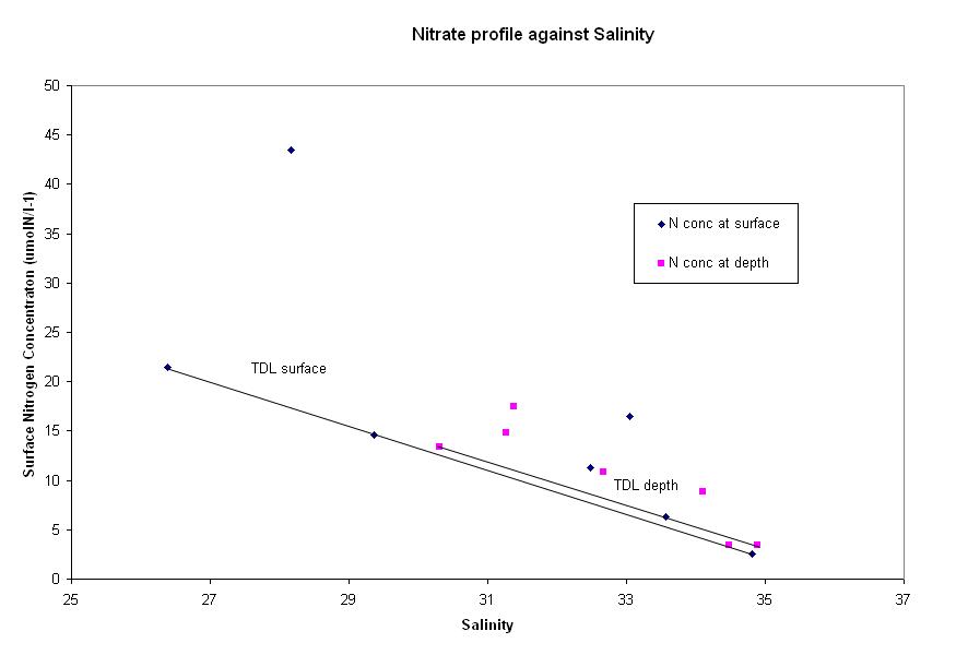
Nutrients Nitrate - The graph above shows
nitrate concentration at the surface and at depth. The data
shows mainly nitrogen addition to the system. The most extreme addition is seen
at a salinity of 28, which is
located downstream of the river Lynher. This may have been a possible source of
nitrate from the boats or houses nearby, which are also surrounded by fields.
However, it would have to be a major source to create the degree of divergence
seen by a concentration of 43.5 umolN/L-1 (it could very well be an anomalous
result). The other extreme point at a salinity of 33 is situated just downstream
of a large oil refinery which would account for the rise in nitrate. The data taken at
depth also shows non-conservative behaviour, as addition is taking place,
suggesting that the estuary is well-mixed. This is supported by the
corresponding CTD data. Phosphate - The estuarine mixing diagram shows non-conservative behavoiur dominating, with little or no relation to salinity. The phosphate curve does not keep to the theoretical dilution line (TDL). The majority of points do not keep to the line. This is more exaggerated in the lower salinity regions of study. Points of phosphate concentration above the TDL indicate that there is a likely addition of phosphate to the estuarine system. Phosphate concentrations are very easily influenced by anthropogenic activity with regard to addition in the water column. When viewing the EMD which is combined with the group 2 rib data. There is a large deviation from the TDL indicating addition of phosphate. The profile does however lead one to believe that it is possible that these points are outliers. However it is also possible that it corresponds to a sewage works as noted by a similar spike in group 3 rib phosphate data. The group 2 rib data also corresponds with group 3 rib data to show that not just addition, but removal of phosphate is apparent in the lower salinity regions of the estuary. Removal is actively removed by flocculation biological removal and interaction with sediments. Flocculation only occurs up to salinity of approximately 10. In higher salinity regions of study, phosphate shows that addition occurs. On comparing the phosphate concentrations between the upper and lower layers of the water column, the marking of TDL’s could lead one to believe that removal occurs in the lower layers of the water column and addition in the upper layers. It can be assumed that as the points are overlapping, there can be no conclusion as to the behavior of phosphate in the water column Silicon - The estuarine mixing diagram showing conservative behaviour for silicon (in the diluted form of silicate) demonstrates a clear correlation with just two sites showing signs of addition. As would be expected the lower salinity regions show a removal of silicate whereas this graph, which was taken from regions further offshore, show two sites with unusually higher concentrations. At site five (as shown on the graph) the data was taken opposite the River Lynher where the more nutrient rich freshwater would have a direct affect on the nutrient concentration. With the catchment being subjected to heavy rainfall a few days before, surface runoff coupled with increased leaching (causing a high nutrient concentration) would largely contribute to the freshwater input. Equally at site 2, the sample was taken downwater of a factory which could be having an affect on the natural processes which regulate the addition and removal of silicate on this environment. Chlorophyll - This graph shows that higher
concentrations of chl a are found further upriver, in both top and bottom layers
of the water column. This is not surprising, due to the increased nutrient
levels found higher in the estuary. Chl
a levels are higher at the surface, ranging from ~4µg/L to ~10µg/L, whereas at
depth, the range is much lower ~2µg/L to ~8µg/L. This was expected, as the phytoplankton bloom will not be found
in the aphotic zone of the water column. However, this cannot be seen in two
distinct layers on the graph, as the salinity also varies throughout the water
column, with the lower salinity at the surface. This is to be expected with
freshwater outflow from the River Lynher overlying the more saline and therefore
denser seawater.
|
| Fig. 34 - Nitrate mixing diagram | |
(Click to Enlarge) |
|
| Fig. 35 -Phosphate mixing diagram | |
(Click to Enlarge) |
|
| Fig. 36 - Silicon mixing diagram | |
(Click to Enlarge) |
|
| Fig. 37 - Chlorophyll against salinity and depth |
|
Zooplankton The number of species of zooplankton increases steadily down the estuary, from 4 to 12 species. This coincides with what has been found in previous samples, ie in the ribs data. This is probably due to the greater number of saline species than freshwater species being imported into the estuary with the flood tide. Copepods are again the dominant species in the sample furthest towards the head of the estuary, with an increase in dinoflagellates and cerripedes, moving to an increase in mysids and medusae and resulting in a diverse community majoring in copepods and cerripede nauplius. There is not too much difference between the total number of species at sites 8 and 14, as they are only 1.3km apart, whereas the other sites are larger distances apart. However, there are relatively large numbers of very different species found at sites 8 and 14, despite the close distance between the two. This suggests that the zooplankton are found in patches, grazing on particular blooms of phytoplankton, and not found evenly distributed throughout the estuary. Phytoplankton The distance each site was from Calstock was used to observe a pattern in Phytoplankton relative abundance. Calstock is a small village up the river Tamar, it would thus be a source of human waste and general chemical runoff.The
Phytoplankton relative abundance is dominated by Diatoms at all sites, never
going below a 90% share of the abundance. At sites 3,14 and 8 Diatoms make up
100% of the measured abundance. These 3 sites happen to be the closest to
Calstock in the order above. Therefore from this it would seem that Diatoms are
more tolerant of extreme conditions such as chemical waste and in fact the
reason for their degree of abundance is that they thrive on increased nutrients
from the waste and out-compete other species. There
is a steady increase in Ciliate abundance the further from Calstock you get,
reaching a maximum of 10% 22.9 km away. This is either due to an intolerance to
the degree of waste closer to Calstock or because the Diatom dominance is no
longer as strong, allowing room for growth. However after Gp3s3 there are no
Ciliates present in the sample. There
is also a similar gradual increase in the case of the Dinoflagellates, beginning
26 km away from Calstock. These results are a clear sign of horizontal zonation
dependent on the distance the area is from Calstock. Niches seem to be formed,
shown by the rise and then sudden drop in Ciliate numbers. This zonation is
especially apparent when you consider the Terschelling data showing
Dinoflagellate dominance of the degree Diatoms did on the
|
(Click to Enlarge) |
| Fig. 38 - Relative Zooplankton Abundance | |
(Click to Enlarge) |
|
| Fig. 39 - Relative Phytoplankton abundance | |
| GPS at start: 50˚
20.7063N |
Aims
Three sites were
initially chosen to scan, but due to errors of the side-scan computer creating
time-delays, only two of these were sampled. At the first site, four transects
were run for one nautical mile, parallel with the western end of the breakwater,
with 50m overlays, to produce a complete map of the area. At the second site, four
transects were chosen, but were altered to slightly further offshore upon
arrival, as the depth (~7m) was too shallow to avoid damaging the fish.
|
||||||||||
(Click to Enlarge) |
|||||||||||
| Fig. 40 - Transects for 1st geophysics plot | |||||||||||
| GPS
at finish: 50˚ 20.1345N |
|||||||||||
| GPS at start:50˚
18.0009N |
|||||||||||

(Click to Enlarge) |
|||||||||||
| Fig. 41 - Transects for 2nd geophysics plot | |||||||||||
| GPS
at finish:
50˚ 18.9866N |
|||||||||||
|
Results On the 6th of July of 2004, a side scan sonar survey was carried out, covering an area of approximately 1800 metres by 200 meters, just inshore of the Plymouth Breakwater. Four transects were completed, incorporating several interesting features of the sediment bathymetry. The plot is shown in figure 42. The first
notable feature found was the base of the breakwater itself. Both ends of the
breakwater were scanned and showed up on the plots, and these are represented on
the plotted diagram by a green colour. A transect close enough to the breakwater
was not completed therefore the entire length was not plotted, but both ends are
clearly shown. Surrounding these ends are areas of coarse-grained sediments.
These sediments have been deposited by water flows that are slowed by the
presence of the breakwater itself, and thus can no longer support its sediment
load in suspension. Also found was some bedrock that was exposed above the
sediments behind the breakwater, shown in black, along with the base of the
moorings used by the large Naval vessels that anchor in this area, as well as
the base of the fort built behind the breakwater during the first world war. |
Fig. 42 - |
The main point
of this investigation, as described in earlier sections of this website, was to
look for evidence of sediment deposition by the flow of water that eddies back
upstream on ebb tides at the western side of the breakwater. This was
investigated because, using our ADCP data on the ebbing tide, evidence was found
of a back eddy that was carrying much less sediment than the main flow. At this
time of year, such occurrences would not normally be happening, but due to the
high rates of precipitation that occurred prior to and during our investigation,
there were raised levels of suspended sediment in the water column. The findings
were not entirely as expected.
It was hoped
that there would be a large amount of sediment deposition inside of the
breakwater, but this was not apparent from the scan data. However, evidence of
sediment deposition was found upon two large-scale bedforms. These bedforms were
set further back from the breakwater than was initially expected. The sediment
appears to have been deposited on top of a scour feature that has incised into
the sediment. This incision was estimated to be approximately 1 meter. Within
the main scour, smaller scours were noted and are illustrated on the diagram.
The two main scours are approximately 360 meters in width at the widest point
found by this survey. The smaller scours are 10 to 20 meters long and appear to
have formed around a nuclei of some sort.
|
A grab was taken in the middle of the eastern most scour feature at a position of 50°20.179N, 4°08.748W to find any evidence of sediment deposition. Figure 43 shows our collected sample. There
is a thin layer of very fine, brown sand, which has been deposited on top of
thick layers of black muds, which become anoxic with increasing depth. It was
concluded that the brown sands on the surface was the sediment that was
suspended within the water column during the investigation on
|
Fig. 43
- |
This study
extended from 0 salinity at the head of the estuary, out to 34 salinity at E1,
and links the physical processes over the two week period with changes in the
biological, chemical and sedimentary processes.
The
survey of the upper estuary showed evidence of a salt wedge during the incoming
tide, as well as temperature profile, with a change of 0.5°C from the warmer
riverine water to the cooler estuarine waters. The nutrients showed very
different results: Silicate showed non-conservative behaviour, with removal in
the upper estuary probably due to uptake by diatoms. Phosphate also showed
non-conservative behaviour, with both addition and removal associated with areas
of past and present industrial use. Nitrate showed slight addition in the upper
estuary, with slight removal in the lower estuary due to uptake by plankton as
well as de-nitrification which reaches a maximum during summer. The plankton
data showed an inverse relationship between the zooplankton and phytoplankton
due to grazing. There is a difference in species dominance throughout the
estuary. Diatoms show dominance in the upper estuary, with 75% of the total
abundance, where Dinoflagellates dominate in the lower estuary, with 90% of the
total abundance. Copepods tend to be the dominant zooplankton species throughout
the entire estuary.
The breakwater
appears to have a significant effect on the flows in the Sound and the
surrounding channels. During the ebb tide, observations of the ADCP backscatter
suggest a reversal of flow direction inside the breakwater, with turbulent
mixing and scouring of the seabed occurring.
During the
period of this study there was a large amount of precipitation for this time of
year. Consequently there was a larger quantity of suspended sediment within the
freshwater source. This increase in sediment lead to previously unobserved
deposition of fine grain sediments on top of these scour features, themselves
also previously unseen on side scan surveys.
The offshore survey showed a phytoplankton bloom
extending from the mouth of the estuary, offshore to a water depth of 50 meters,
as well as various other areas of backscatter indicating plankton maxima at
depth. At the E1 monitoring station we recorded a very distinct thermocline at a
depth of 29 meters, with fluorescence maxima (4.0 micrograms per litre) at 28
meters. This fluorescence maxima coincided with a backscatter peak from the ADCP
data indicating zooplankton grazing. The fluoresence maxima occurs just above
the thermocline because nutrients leach slowly through it, enabling the
phytoplankton to take advantage of the available nutrients. In the zooplankton
net we took in a vertical plane through this backscatter peak we found a huge
abundance of large unidentified nidrian plankton, which were approximately 2cm
in diameter. Backscatter peaks were also identified above the two peaks of
Eddystone Rocks which were covered; this coincided with a decrease in the depth
of the chlorophyll maxima which was noted on the miniBAT transect in the same
area.
Kiorboe,
T. (1993). Turbulence, phytoplankton size, and the structure of pelagic
food webs. Adv. Mar. Biol. 29, 1-72.
Miller, C.B. (2004). Biological Oceanography, Blackwell. pg 120.
Holligan P.M. et al. (1984). Photosynthesis, respiration and nitrogen supply of plankton populations in stratified, frontal and tidally mixed shelf waters. Marine Ecology-Progress Series. Vol. 17:201-213.
Fretter,
V and Shale, D. (1973), Seasonal
changes in the population density and vertical distribution of prosobranch
veligers in offshore plankton at
Dyer, K.R (1994). Sediment Transport Processes in Estuaries. In Geomorphology and Sedimentology of Estuaries Perillo, G. M. E. (ed) Elsevier
Tattersall G. R, Elliot A. J and Lynn N. M. (2003) Suspended sediment concentrations in the Tamar estuary, Estuarine Coastal and Shelf Science, 57, pp 679-688
Bautista, B. et al, (1994), Temporal variability in copepod fecundity during two different spring bloom periods in coastal waters of Plymouth, Journal of Plankton Research, Vol.16 no.10, pp.1367-1377
Fretter,
V and Shale, D. (1973), Seasonal
changes in the population density and vertical distribution of prosobranch
veligers in offshore plankton at
Maddock,
L. et al, (1989), Seasonal and year-to-year changes in the phytoplankton from
the
