The Group

(From top left to bottom right) 

Dan "Why Did I Ever Buy Steel Toe-Caps" Miners, Joseph "Merman" Rolfe, 

Liam "The Man, The Mission" Missin, Matthew "Best Break-up Story Ever" Donnellan, 

Mike "Plunder Yo Booty" Smith, Chris "Sacrifice Him to Our False Gods" Osowski, 

Ana "I'm not English" LeMarie, Susan "Where Did That Wave Come From?" Collins, 

Victoria "I love Sigma Plot" Venturini, Clare "Evil Carrot" Stratford

Introduction

Over two weeks, from the 23^rd June to the 7^th July 2004 , Group 12 investigated riverine, estuarine, coastal and offshore environments in Plymouth , with the aim of gaining an holistic overview. The study area comprised of the River Tamar, two sub-estuaries, namely the Tavy and the Lynher, Plymouth Sound and the offshore waters.

A naturally occurring breakwater acts as a partial barrier at the lower reaches of the Tamar estuary; the upper reaches are situated at Calstock. The Tamar river and its tributaries provide the main input of fresh water to the estuary system. The main Tamar estuary is a ria (a drowned upland river valley) and the waters of the estuary are temperate and partially mixed. The estuary is flood dominated, with semi-diurnal tides.

Geophysics - Nat West II

 BREAKWATER TRANSECT:

            Two parallel tracks (50m separation) between:

 TAMAR (OFF KINTERBURY) TRANSECT:

            Four parallel tracks (50m separation) between:

 TAMAR (OFF KINTERBURY) GRAB:

            One Van Veen Grab at:

 TAMAR (ABOVE THE BRIDGE) TRANSECT:

            Two parallel tracks (50m separation) between:

            and

Terrestrial Geology

On the morning of 24^th June 2004 at 0830-1030 UTC, previous to the geophysical survey of the Plymouth Sound and the Tamar Estuary, the geological land features of Heybrook Bay were observed. Those observed were fault lines and fractures caused by the tectonic movement of the surrounding area and the dip/stike and alignment of the folds found therein. High tide was at 0940 UTC with a tidal height of 4.71m.

Preliminary results                                                                                                                                                                                                                    

Log of the cliff face:

Figure 1 - Small Section of Heybrook Cliff (Click to enlarge)

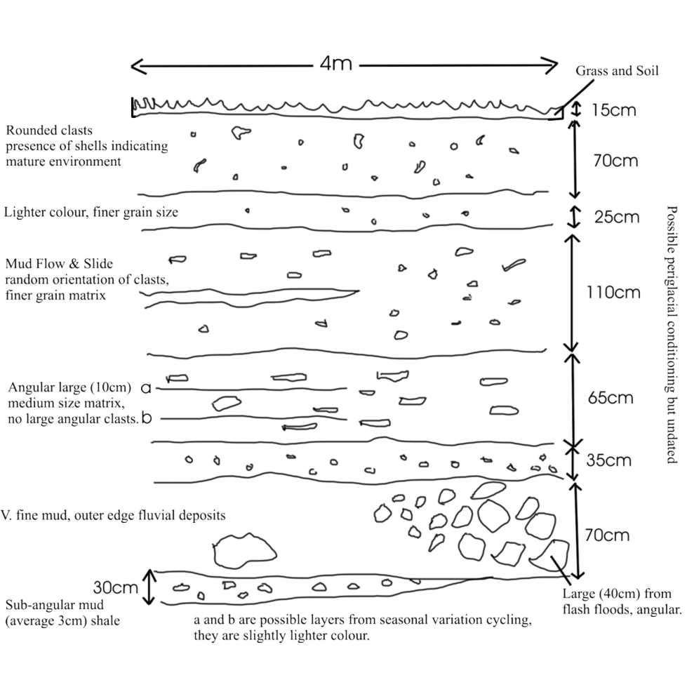The section studied (Figure 1) covered an area of 4m wide and 4.2m high.  The bottom section is muddy and characteristic of an outer fluvial environment. The presence of boulders in this section indicate a high energy environment that is probably caused by flash floods.

The next section is mainly muddy with some shale. A section with larger clasts up to 10cm follows indicating a medium energy environment. Above this section the clast size decreases but the random orientation of these suggests that they were deposited by mud flows or mud slides. There are other theories attributed to the formation of this section, although none have been published. The random deposits may be associated with the melting of the ice sheets that covered the north and middle of the U.K.

The sequence then moves into a lighter colour fine grained sediment. The last sequence is characterised by subangular clasts and many shell fragments. the shells suggests a marine depositional environment compared to the previous fluvial ones. The angularity of the clasts in most of the cliff indicates their poor maturity.    

   Figure 2 - Geological Features of Heywood Bay, South from Shoreline

Dip and strike of beds:

The beds in this area strike in a SW-NE direction and dip SE with an average inclination of 55°.

Fold:

The outcrop of fold was found at 49240E/48780N. It was identified as a recumbent antiform fold plunging SW with the hinge line pointing 220°.

Fault:

A dextral fault cuts through the fold off-setting it by 5 meters. The direction of the fault is 117°. Due to the high tide, further investigation of the fault was not possible.                                           

Side Scan Sonar                                                                                                                 

Offshore Geology  

Figure 3 - Fault Map of Plymouth (Click to enlarge)

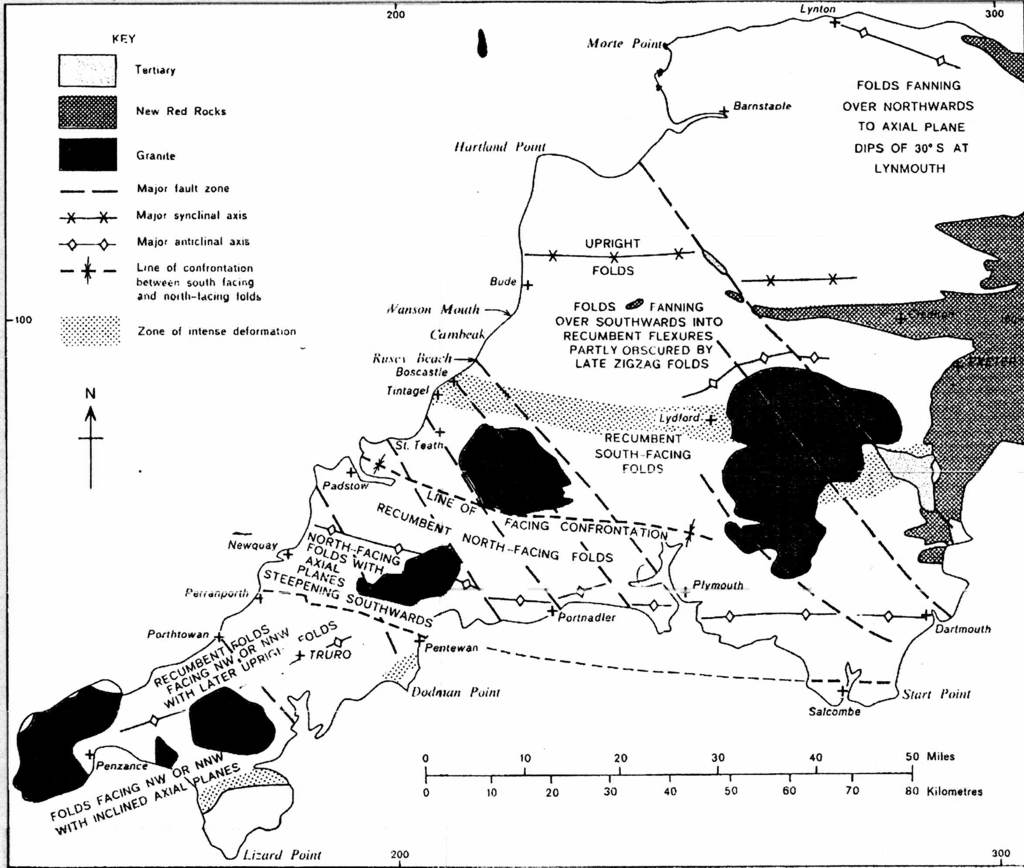The preliminary objective was to look at the near shore geology off Renney point. A major fault was found from the side scan sonar and later identified using geology maps (NERC, 1985) (fig. 3) as the Rusey fault.

The two tracks carried out ran from 248600 – 245700 (Easting scale) along a constant Northing of 49340. The other track ran parallel to this and was the same length but 50m North.

The two tracks showed similar features; a 370m wide rocky area beginning at 246280 and extending to 245760. The bedding planes in the region have a N/NE strike direction similar to that observed at Renney point. The rock covers some crevices and boulders which cause the depth to vary across the region. The average depth relative to the sonar fish was 13.7m although dips and boulders were measured and found to be 0.3 to 0.95m higher or lower. The change in bathymetry is probably due to the softer rock, which erodes more rapidly, interlaying harder more resistant rock.

Figure 4 - Track-plot for the Breakwater Scan

Figure 5 - Bathymetric Profile of Plymouth Sound (Click to enlarge)

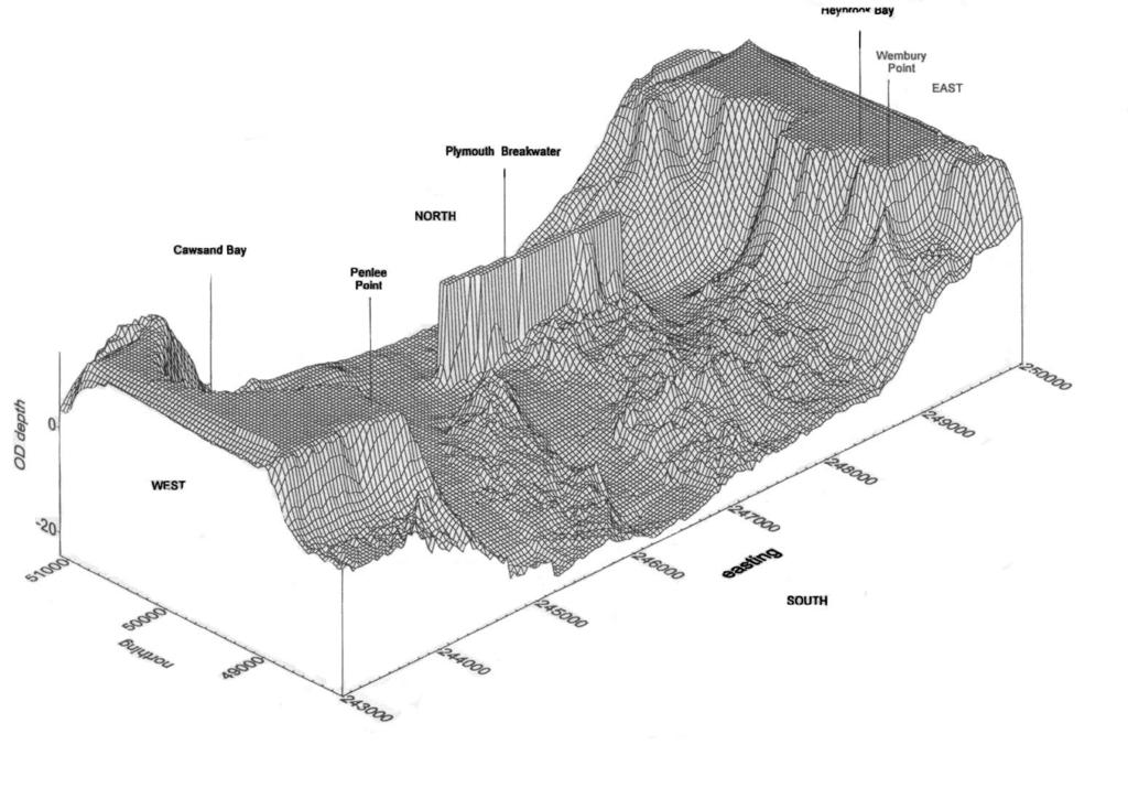At 246280E the depth of the seabed increased to 19.4m, which corresponded to a transition of the seabed from rocky outcrop to sediment. This sediment region extended for 500m and included areas of sand ripples with wavelengths of ~1m. As the wavelength was relatively small the height of the ripples could not be determined as the shadow zone associated with each ripple was not large enough to be measured. The direction and clear bifurcation of the ripples would suggest that they are wave generated by the storm waves coming in from the SW. This can be implied because the depth of the area means that only waves of storm proportions would be able to influence the seabed. Energy rebounded from the breakwater may also contribute. Even so, there were small strips of ripples present which could not be wave generated due to the orientation and lack of bifurcation. 

At 246900E the exposed bedrock re-emerges, although with some sediment cover suggesting a strong current to move sediment over the rock. This region continues to the end of the track, and is similar to the section at the start. A scour mark (15m x 10m) was seen at 246920E and 49380N which may be due to a strong localised current emerging from behind a boulder nearby. The plunging fold could explain the greater sediment cover as sediment would collect in the lower lying seabed.

In summary, the area is a high energy environment with a major fault running through it at a bearing of 150°, identified as the Rusey fault (fig.3). The recumbent fold has subsequently been divided by faults, on a major and minor scale similar to Renney point (5m dextral movement) and Rusey fault (15m dextral movement). The sandy channel between the two rocky regions could be one of three palaeo-river channels,  well known geological characteristics of the region (Plymouth Bathymetric Survey 1997) and links to the fluvial generated debris seen in the cliff section on Renney point and the associated sea level change (fig.4).

Limitations:

When interpreting the side scan sonar data a 60 second discrepancy was observed between the two transects. As they were continuous, this was a 30 second discrepancy on each. It was determined that this was due to chronological impairment between the different hardware, namely the GPS system and the side scan sonar system.

The extent of the time delay was quantified by referencing fixed points on the sonar plot to times when they were passed on the GPS plot. The fixed points used were the Tamar Bridge turrets and when frequencies were switched between 100Hz and 500Hz.  The time difference observed by this method, was 20 seconds.

Therefore, the GPS times were altered by the observed 20 second discrepancy; hence the times on the track plots are the GPS plus the adjusted time.  

River Geology

After examining the offshore area it was decided to head for the upper reaches of the river Tamar. This was for two reasons:

Previous study of the Plymouth Sound had been performed by other groups so collecting data again from these sites would not yield any new results.

The area of study was the intersection between the river Tamar and the Lynher River.

Results:  

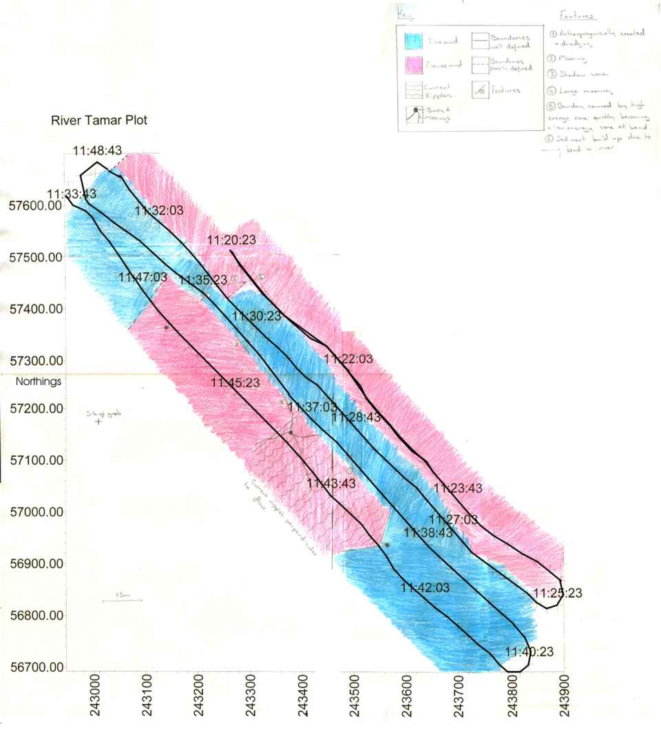
Figure 6 - Tamar River Plot

Our survey of the area began at 11:20 UTC, the summary of findings is as follows:

The complex distribution of sediment grain size can be seen as a result of the two converging rivers along with the flood and ebb of the estuary. The larger grain sizes are as a result of higher energy either from the rivers joining or the bend in the river.

Ripples of a wave length 5.47m between 243500E / 56970N and 243350E / 57160N produced by the currents in the estuary.

Anchor chains which hold the large special buoys in position can be observed. Using the chains located at 243370E/57160N ( 10:37:50 ) two chain marks can be seen on the side scan. This has a few possible explanations; firstly these marks could be as a result of the ebb and flood of the estuary, however, there is no sign of disturbance between the two marks which you would expect if the chain had been dragged along the bottom therefore it is more likely to be two separate chains to hold the buoy more securely. This would need to be studied again to determine the true meaning of the side scan sonar readout.

The Van-Veen grab was used at 11:46 UTC at position 50°23’.659N/004°12’.468W (57175N, 243050E) next to the No .9 yellow mooring. Water depth was 17m. This determined what the sediment was on the western side of the side scan readout.

Composition: Thick, poor quality muddy sediment with a thin anoxic layer 

Contains empty Mussel shells, Spartina weed and Polychete worms (about 10cm long). The thin anoxic layer was about 5cm below the surface and had a slight odour.

References:

South West England 1985 British Geological Survey (NERC)

Plymouth Field Course Geophysical Practical Handout.

Back to the top

Estuarine - R.V. Bill Conway

STATION 1:

STATION 2:

STATION 3:

STATION 4:

STATION 5:

STATION 6:

STATION 7:

STATION 8:

STATION 9:

STATION 10:

 STATION 11:

Figure 7 - ADCP                     Figure 8 - CTD

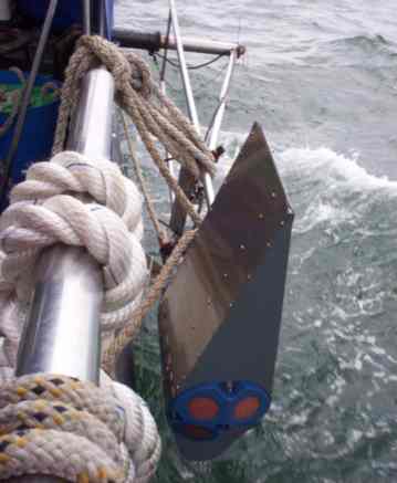
On the morning of June 28th 2004, from 0830-1530 UTC, the Research Vessel Bill Conway was used to sample 11 different stations using a CTD with Niskin water bottles and ADCP (Fig. 7 and 8).

Previous results from group 6 on June 27th showed a backscatter anomaly (an area of high backscatter) at position 1 (Fig.8). It was decided to investigate this anomaly and carry out three transects around where the anomaly was first seen, in an attempt to explain the position and composition of it. The position of the three transects are shown below in figure 8.

Figure 8 - ADCP sample triangle (Click to enlarge)

When the ADCP data was analysed, an anomaly was seen on the first transect, assumed to be the anomaly observed the day before. The fluorometer readings were constant, therefore the backscatter was probably not due to zooplankton but possibly suspended load. It was not seen on the other two transects suggesting the anomaly was not concerned with the River Lynher or the flow from the mouth of the estuary. Figure 9 shows the anomaly seen at Position 1.

                                                                                                                Figure 9 - ADCP Backscatter Position 1 

The area where the anomaly was seen was scrutinized and it was discovered that a bank extended out from the western shore to the middle of the channel reducing the depth of the channel by five metres, effectively forming a barrier that the current had to move over. It was therefore deduced that the anomaly was due to scouring by the current, increasing the sediment load and hence increasing the backscatter intensity.  This is confirmed with the aid of the transmisometer readings (Figure 10).

Normally the program "CTD Analysis" would be used to process these raw data into depth interval averaged, but due to a bug it was unable to analyse certain CTD readings. This can be seen in the station 4 and 5 graphs, as the raw data had to be used, hence the irregular chart lines.

x:\group12\data\Bill Conway (Estuary)\ADCP

 Figure 10 - Transisometer Readings from Stations 3,4 and 5 (Click to enlarge)

x:\group12\processed\Bill Conway (Estuary)\CTD\Excel\alldata(fl).xls

ADCP Profile – Breakwater:

ADCP transect ran across the sound just behind Plymouth breakwater from position 50° 20.593N/004° 09.906W to end position 50° 20.568N/004° 07.840W. The breakwater runs from 50° 20.042N/004° 09.551W to 50° 20.004N/004° 08.292W.

The velocity magnitude profile of the water column, measured by the ADCP, showed a very well mixed water column. There were no major changes to the water column along the track.

The flow direction around the breakwater showed most water flow into the sound coming through the western channel as the direction of flow was to the North East. Direction of flow through the eastern channel is predominantly in a southerly direction, suggesting the flow out of the sound occurs through the eastern channel.

                                                                                                                                                   Figure 11 - Breakwater Track Plot

 X:\group12\Data\Processed\Bill Conway (Estuary)\ADCP\6021r.r00

As seen in figure 11 above, flow behind the breakwater also appears to be southerly. This is due to the breakwater preventing northerly flow from the open ocean  into the estuary. Therefore, the only flow in this region is from the river outflow in a southerly direction out of the estuary. Even so, flow behind the breakwater is reasonably low.

Silica

The geology of the area  sampled, from the River Tamer out to the Sound, alters from Upper Devonian to Lower Devonian sedimentary rock respectively. The silica present in these rocks are subjected to chemical weathering leading to dissolution and erosion (Wollast, 1999).  Dissolved silica represents a dominant species in river water as undissociated silicic acid: SiO₄H₄. 

Not all the dissolved silica present in estuaries is  transported to the sea as it is largely affected by phytoplankton activity in the coastal zone. It is also affected by continual deposition and re-suspension processes which in turn are affected by river discharge.

Chlorophyll

Figure 12 (Click top Enlarge)

Figure 12 shows the chlorophyll concentration throughout the estuary. The maximum concentration occurs in the upper estuary , this corresponds to a large reduction in silica concentration in the upper estuary, this drop in silica corresponds with an increase in the amount of diatoms, which utilise silica for test formation.

X:\group12\Data\Processed\Bill Conway (Estuary)\Biology\Chlorophyll\chlorophyll processed.xls

Figure 13 - Salinity vs Silica Concentration (Click to enlarge)

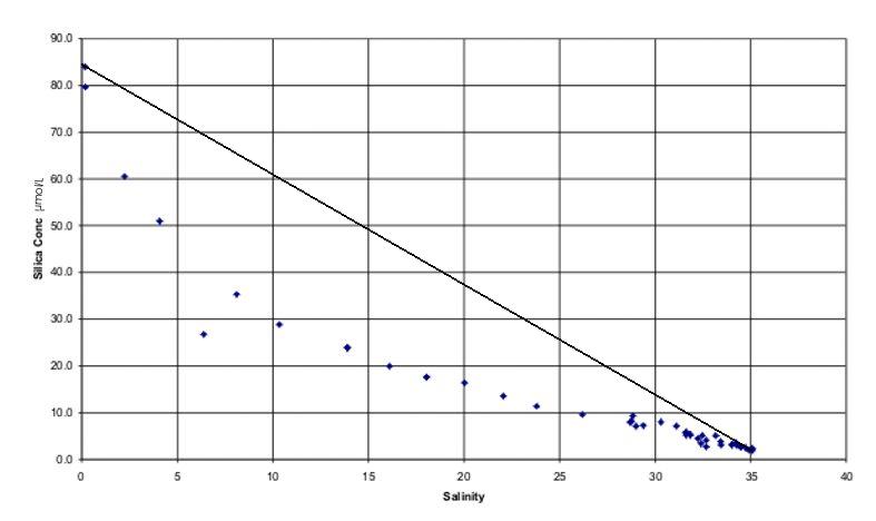
The mixing diagram shows that silica behaves non-conservatively with removal occurring between the two end members.  The highest concentration of silica corresponds to the riverine end member sample. Concentration decreases from 84µmol/l to 28µmol/l over salinities 0-6, then rises to 36µmol/l at salinity 8 before decreasing to 2µmol/l at the seawater end member. This removal is assumed to be due to the assimilation of the silica by diatoms. 

The maximum rate of change of silica removal is equal to 8.5µmol/l/psu at a salinity of circa 6. This is also the salinity where the chlorophyll concentration and number of diatoms are at a maximum. After this the concentration of silica decreases to meet the marine end member in a mainly linear fashion.

X:\group12\Data\Processed\Bill Conway (Estuary)\Chemistry\Silica\silicaconway.xls

Figure 14 - Chlorophyll Vs Silica (Click to enlarge)

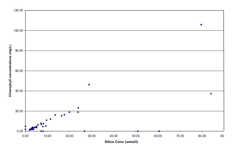
Figure 14 shows an apparent linear relationship between chlorophyll and silica concentrations. Chlorophyll increases as silica increases due to the diatom population requiring silica for cell growth (also being the dominant species in this situation) and hence being limited in numbers by the abundance of silica. 

X:\group12\Data\Processed\Bill Conway (Estuary)\Chemistry\Silica\silicaconway.xls

 Figure 15 - Phytoplankton Concentrations (Click to enlarge)

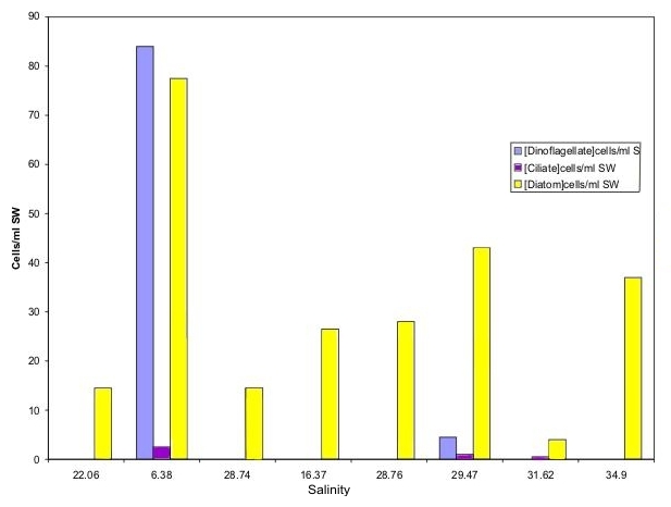
Figure 15 shows the concentration of phytoplankton through the estuary. It explains the presence of a chlorophyll spike at a salinity of 6.4, corresponding to a spike of dinoflagellates and diatoms. Diatoms, which have a siliceous cell wall, account for the removal of silica as shown in Figure 14, which also occurs at a salinity of 6.38. Cilliate cells remain at a very low level thorough the system only peaking at 2.5 cells/ml Seawater which is also seen at a salinity of 6.38.

X:\group12\Data\Processed\Bill Conway (Estuary)\Biology\Plankton\zooplankton.xls

Plankton abundance & diversity in the river Tamar and Plymouth Sound

                                                                                              Figure 16 - Plankton Abundances (Click to enlarge)

X:\group12\Data\Processed\Bill Conway (Estuary)\Biology\Plankton\zooplankton.xls

Plankton trawls were carried out using 200µm mesh size plankton net, both from the RV Bill Conway.   

Bottle 13 from 50°24.559N / 004°12.201W was brackish water of salinity 20.04. From the pie chart (Fig. 16), group abundance here is low with 85% composed of the crustacean Cirripede nauplius. The second greatest abundance is seen in dinoflagellates although they only compose 9% of the total zooplankton population. Diversity is very low which can be attributed to the stressful conditions caused by the relatively low salinity.

The second pie chart shows the species diversity from bottles 1 & 2 carried out at 50°25.480N / 004°12.183W where salinity was 30. Composition of the Cirripede nauplius species has dropped to 58% with dinoflagellates composing 23% of all species; the salinity here is higher, conditions are less extreme, and other groups can compete with the Cirripede nauplius.

The end member trawl taken near the break water at 50°20.042 N / 4°09.551W shows the greatest number of groups in the zooplankton count; 65% of all species collected here were copepods, 13% dinoflagellates and 6% gastropods. The previously dominant Cirripede nauplius species now only compose 2% of the sample.

Phosphate Behaviour along the R. Tamar:

Figure 17 - Theoretical Dilution (Click to Enlarge)

Figure 17 shows the general trend of an addition-removal curve.  This trend can be confirmed by looking at group 1 and 8’s data, found at x:\group1\smallboat\processed data\group4 data\g4PO4 and x:\group8\billconway\nutrients\phosphate

                                                                                                                                                                                     Figure 18 - Phosphate against Salinity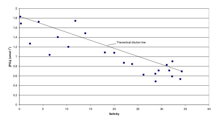 (Click to enlarge)

At low salinity phosphate concentrations were at a maximum, with a concentration of 1.8µmol l^-1.  Phosphate is added in the upper estuary, suggesting that phosphate input is from terestial sources.  The observed land use in the upper estuary is predominatly farmland, this together with the high rainfall during the sample period may have increased the amount of phosphate being washed of the land.  Addition may also be due to inputs from the River Lyhner and the River Tavy

At a salinity of approximately 17, the dominant processes in the estuary is removal, this is probably due to removal in the lower estuary by phytoplankton.

                                                                                                            X:\group12\Data\Processed\Bill Conway (Estuary)\Chemistry\Phosphate\phosphate.xls  

                                                                                                                  Figure 19 - Station 11 Phosphate/Salinity (Click to enlarge)

To establish the relationship of phosphate and salinity with depth a vertical profile was plotted for station 11 shown in figure 19. This station was on the eastern side of Plymouth Sound at position 50º 20.642N / 004º 08.140W. This profile shows that phosphate decreases with depth whilst salinity increases. The surface is fresher riverine water, undercut with saline marine water with the same pattern as the river profile seen in Plymouth Sound - phosphate concentration decreases with increasing salinity. Depth profiles for other stations appear to show the same relationship.

Nitrate:                                                                                                                    X:\group12\Data\Processed\Bill Conway (Estuary)\Chemistry\Phosphate\Phosphate.xls

Nitrate concentrations were determined from water samples taken from the River Tamar at 50°29.750N / 004°12.411W, down to the breakwater in Plymouth Sound at 50°20.642N / 004°08.140W. The calculated concentrations were plotted against salinity to determine the theoretical dilution line (TDL) and behaviour of nitrate along the studied transects. (Fig.18).  

Figure 20 - Nitrate against Salinity (Click to enlarge)

Along this horizontal profile of surface samples, the river end member (salinity 0.16), had a concentration of 146μmol/l, while at the saline end member (salinity 34) the concentration was 4.8 μmol/l. The behaviour is non-conservative as the points lie below the TDL. This suggests removal of the nutrient possibly by phytoplankton.

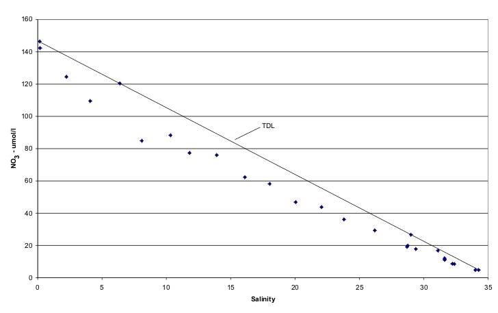
As shown in figure 15, at a salinity of 6.38, a high concentration of dinoflagellate cells are found. This appears to correspond to the greater decrease in nitrate at the same salinity, suggesting that the depletion is due to biological factors. The rate of change is equal to 8.5µmol/l/psu as it was for the silica.   

X:\group12\Data\Processed\Bill Conway (Estuary)\Chemistry\Nitrate\Nitrate.xls

Back to the top

Offshore - Terschelling The The trip on the Terschelling was taken on the 2^nd July 2004 from approximately 08:40UTC to 14:00UTC. High water was at 17:50UTC, low at 11:20UTC and there was a strong south-westerly of force 6 blowing (having fallen since the storm the night before). As such, travelling far outside Plymouth Sound was disregarded and the following plan was made:  

Station 1 and 7

Figure 20 - Station 1 and 7 Silica Concentration (Click to enlarge)

This was the first site to be sampled at 08:20UTC. It was sampled again at 12:55UTC and referred to as station 7. Station 1 and 7 have a similar profile for silica concentration (Fig 20.) It increases steadily with depth down to 7m for station 1 and 6m for station 7, after which a decline in concentration is observed. However, the data obtained for station 7 are all consistently higher values than those at station 1 by about 1.4µmol/l.  This is probably due to the change in salinity at these different sampling times, caused by them being either side of low water (11:20UTC).  

X:\group12\Data\Processed\Terschelling (Offshore)\Chemistry\Silica\silica.xls

Subsequently, measurements at station 1 reveal the water is more stratified than at station 7, where values are spread over a larger range. The surface water has a lower salinity than at station 1, and the water at depth has a higher salinity than at station 1. 

Figure 21 - Salinity vs Depth at station 1 (Click to enlarge)                                                                                                       Figure 21 - Salinity vs Depth at station 7 (Click to enlarge)

X:\group12\Data\Processed\Terschelling (Offshore)\CTD\ctd.xls

Figure 22 - Phosphate and Phytoplankton vs Depth at station 1 (Click to enlarge)

At the surface, phosphate concentration is double compared to station 7. Chlorophyll concentration graphs for each station help account for these values of phosphate.  For station 1 phosphate decreases from the surface down to a depth of 7m while chlorophyll concentration increases.  At 10m phosphate starts to increases and chlorophyll decreases slightly after 7m.  At station 7, phosphate concentration increases from 0.25µmol/l at the surface to almost 0.3µmol/l at 6m, from which point it continues to increase at a greater rate until 9m where it reaches 0.37µmol/l.  When compared to chlorophyll the inverse relationship is present again.  This could be due to the lower concentration of phosphate at this site partially limiting the phytoplankton population, thus lowering chlorophyll concentration.  In the surface layer chlorophyll concentration decreases slightly  down to a depth of 6m, due to this apparent decline of phytoplankton, phosphate concentrations increases over this depth.  After which, chlorophyll concentration decreases at a greater rate and phosphate increases as moving further away from the surface, and deeper into the euphotic zone. Cell numbers of phytoplankton at station 7 remain around 70 cells/ml SW down to a depth of 5m, where after they increase quickly to their highest of nearly 150cells/ml SW at a depth of 9m.   

X:\group12\Data\Processed\Terschelling (Offshore)\Chemistry\Phosphate\phyt PO4.jnb

                                                                                                                                        Figure 23 - Nitrate verses Depth for Stations 1 and 7

Nitrate concentration at station 1 is overall lower than the values found at station 7.  This can be linked back to the salinity graphs for these stations which show station 1 as having fairly good stratification and station 7 as having less saline surface waters and greater salinity of deeper waters in comparison to station 1, thus there is more fresh water at station 7 which would account for the higher readings of nitrate.  At station 1 nitrate concentration increases from the surface to 8m, where after it decreases at a greater rate to the depth of 10m.  The nitrate concentration over depth for station 7 decreases rapidly to 6m, then decreases at a much lower rate to 9m.   These variations could be attributable to extent of mixing of water column, as the expected inverse relationship between chlorophyll and nitrate is not apparent.  This may be due to a lack of data points giving an incomplete overview. 

Some of the data for station 1, including our phytoplankton data was, unfortunately, lost.

X:\group12\Data\Processed\Terschelling (Offshore)\Chemistry\Nitrate\nitrate tech.jnb

Station 2

Station 2 (50°19.792 N, 004°11.334 W) was studied at 09:15 UTC. This station was located at Cawsands Bay and the reason for studying this station was to examine the temporal variation of the water column.

Figure 24  - Thermocline Station 2

Station 2 had a depth 12m and a current of ~ 0.8knts with a flow direction of 225°. Cawsands bay is sheltered by a headland meaning that the winds which were South Westerly , gusting 20knts out to sea were not present and the area was relatively calm. The following describes the results obtained from chemical sampling

X:\group12\Data\Processed\Terschelling (Offshore)\CTD\Excel\allstats.xls

Figure 25 - Silica Station 2

Nitrate shows no change through the top 5m recorded (unknown below this depth as data was lost due to an accident in the lab). The nitrate reading remains constant at roughly 0.6 μM. Silicate increases linearly by roughly 0.25 μM over the 5m depth recorded. Phosphate decreases through the top 5m from 0.45 μM to 0.175 μM and Chlorophyll decreases from 1.75 μg/l to 1.5 μg/l from surface to 5m, then increases to 2.1 μg/l at 10m.

X:\group12\Data\Processed\Terschelling (Offshore)\Chemistry\Silica\Silica.xls

Figure 26 - Phytoplankton Station 2

Phytoplankton increases from 22 cells per ml of seawater to 35 cells per ml of seawater over the first 4m then decreases to ~10 cells per ml of seawater at 10m.

The following describes the physical data obtained from the station.

ADCP: there is a noticeable high backscatter at ~ 5m

CTD: This shows a distinct thermocline at 5.7m

Discussion

Due to the loss of results it is thought that the chemical data may contain substantial errors. The following discusses the above results with respect to each other and tries to put forward some initial ideas as to how they are linked.

The phytoplankton maximum is found in the top 5m of the water column and is believed to be constrained by the thermocline.

Phytoplankton uses nutrients suggesting that the nutrients should decrease with increasing phytoplankton.

What was actually seen is:

 Further

Chlorophyll concentration, which is positively proportional to phytoplankton, appears to be negatively proportional at this station. This requires further investigation but is believed to be error created by the following possible errors.

1. Human error with phytoplankton count
2. Human error with chlorophyll
3. Something else which has not been seen

Station 3  

Figure 27 - Nitrate Station 3

At station 3 the CTD was deployed at 50°18.696N / 004°10.237W and showed the presence of a thermocline and halocline at the depth of 10m.

Figure 27 and 28 show how phosphate and nitrate increase from a depth of 15m. 

Silica increases from a depth of 10m. But it is not possible to know what silica is doing at depth shallower than 10m due to data loss.

X:\group12\Data\Processed\Terschelling (Offshore)\Chemistry\Nitrate\nitrate tech.jnb

Figure 28 - Phosphate Station 3

X:\group12\Data\Processed\Terschelling (Offshore)\Chemistry\Phosphate\Phosphate.xls

Figure 29 - Chlorophyll Station 3

Chlorophyll concentration starts decreasing at 10m and at 15m it undergoes a rapid decline in concentration (Fig. 29). This decrease in chlorophyll and increase in nutrient concentration corresponds to the thermocline depth that does not allow mixing between the upper and lower layer.

Another limiting factor for the growth of phytoplankton at this station is light irradiance, the 1% light depth was measured at 21m from the 7m secchi disc depth.

X:\group12\Data\Processed\Terschelling (Offshore)\Biology\Chlorophyll\chl graph.doc

Station 5.                                                                                                                                                                                            Figure 30 - Thermocline Station 5

Station 5 was offshore at 50°18.5N/4°07.7W, 1050UTC.

Due to the adverse weather conditions limiting the distance from shore, this site was chosen as our off-shore station at which to study the stratification during summer and its effect on biological and chemical aspects.

Station five shows a well stratified water column. By using CTD data, a strong thermocline can be seen at 15m with a change in temperature from 13.5°C to 12.4°C. The secchi depth of 8m allows us to calculate the depth of the euphotic zone as 24m. Water above the  euphotic zone has a  temperature of 13.5°C and salinity of 35.16 while below its 12.5°C and 35.25.

                                                                                                                               X:\group12\Data\Processed\Terschelling (Offshore)\CTD\Excel\allstats.xls

Figure 31 - Phytoplankton Station 5

Due to euphotic stratified waters being exhausted of inorganic nutrients during the summer months (Kiorbe 1993) phytoplankton levels are at their maximum (15cells/ml SW) at, or near the thermocline due to nutrient recycling below. This can be seen clearly on the plots of phytoplankton numbers. Looking at the various data sets for the nutrients analysed at this station a clear pattern is seen which backs this up. The phosphate, nitrate and silica concentrations show an inverse relationship with cell numbers, where an increase in phytoplankton numbers sees a reduction in these nutrients.

X:\group12\Data\Processed\Terschelling (Offshore)\Biology\Plankton\phytoplankton.xls

Figure 32 - Nitrate Station 5

Looking in more detail at phosphate and silica, a sub-maxima is seen at 10m which coincides with the phytoplankton maxima. The high presence of phytoplankton causes a decrease in silicate and phosphate due to consumption. As the nutrient levels become limiting ca.17m the phytoplankton levels also drop, so by 20m there are 13 cells/ml SW.  These data show a spike in both silica and phosphate levels at 10m, the exact reason for this isn’t clear as it would be expected to see a decrease in the levels. The two explanations for this is either that it is an error as the peaks do fit within the error margin set by the error bars, or that the phytoplankton had only recently arrived in the area. However this would require further investigation.

X:\group12\Data\Processed\Terschelling (Offshore)\Chemistry\Nitrate\nitrate tech.jnb

Figure 33 - Phosphate Station 5

This results in a decrease in consumption of nutrients which combined with the rich waters below the thermocline allows the nutrient levels to rise suddenly, this produces a PO4 maximum at 30m of 0.50µmol/l-1. Due to the low irradiance (24m euphotic layer base) the phytoplankton at this depth are unable to reform and utilize the nutrients. So light is a limiting factor. 

It is important to note that the phytoplankton count for this station composed almost entirely of diatoms alone. This is important as they utilize large levels of silica due to the silacious epi/hypotheca which is an important component of their cellular construction.

X:\group12\Data\Processed\Terschelling (Offshore)\Chemistry\Phosphate\Phosphate.xls

Station 6  

Station 6 (50°19.819 N, 004°11.387 W) at 11:51 UTC had a depth 12m and a current of ~ 0.1 (slack) with a flow direction of 190°. Cawsands Bay is sheltered by a headland meaning that the winds, which were South Westerly, gusting 20knts out to sea, were not present and the area was relatively calm. The following describes the results obtained from chemical sampling

It is observed that nitrate decreases from 0.74 μM to 0.67 μM from the surface to 6m it then decreases to 0.53 μM at 8 m. further silicate decreases from 4.2 μM to 1.7 μM from the surface to 6m it then increases to 1.9 μM at 8m. phosphate decreases linearly from 0.36 μM to 3.00 μM from the surface to 8m and chlorophyll increases from 2.8 μM to 3.3 μM from the surface to 6m then decreases to 2.7 μM at 8m.

Phytoplankton decreases linearly from 17.5 to 6.2 cells per ml of seawater from surface to 8m.

The following describes the physical data obtained from the station.

The CTD shows no distinct thermocline with the temperature decreasing from 14.3°C to 13.7°C

Discussion

Again a decrease in phytoplankton and an increase in chlorophyll is seen, it is the believed that the chlorophyll samples are a more accurate representation of the relative phytoplankton in the water column than the phytoplankton count is. 

A major point to be analysed is why is the thermocline more pronounced at 09:15 UTC (Station 2) than 11:50 UTC ?

At 09:15 the tide is hitting the headland and being pushed away from Cawsands Bay meaning the currents in the bay are very slight despite what the closest tidal diamond says. This is backed up by the ADCP data. The closest tidal diamond suggests that the tide is flowing 260°. However the ADCP data suggests it is flowing at roughly 080° This is likely to be a result of eddying within the bay from the slight current which enters it. This produces a very calm, stable environment allowing the thermocline to become distinct as found at station 2. As the tide swings around towards the east it starts to flow into the bay and causes mixing which disrupts the thermocline. This is supported by the ADCP data as the velocity shows the tide flowing in a westerly direction and is more variable due to the increase in velocity even though it is only 1 hour after high water (slack water).

CTD profiles – Station 2, 3 and 4

When Station 2, Cawsand Bay, was sampled a halocline was observed as shown in figure 34. It was decided to track this halocline further out to sea to observe how far the halocline extend and also possibly inferring the reason for it’s presence.     

                                                                                                                                                    Figure 34  - Station 2, 3, and 4 Salinity Profile

                                                                                    X:\group12\Data\Processed\Terschelling (Offshore)\CTD\Excel\CTD.xls

The halocline was still present at Station 3 yet less pronounced.  Once again shown in figure 34, the halocline was even less pronounced at Station 5.  A possible reason for this is that the fresh water present inshore is being held into Cawsand Bay by the strong south westerlies that were present on the day of sampling.  Station 5 was yet further away from Cawsand bay, and as can be seen in figure 34 the halocline is still present but much smaller in magnitude than the previous two stations once again symptomatic of the fresh water being held in Cawsand Bay by the strong south westerlies.  Also it is prudent to note that the depth of the halocline in the water column reduces as it approaches the shore because the salt water is pushed up by the topography ergo reducing the depth of the halocline.

                                                                                                                                                    Figure 35 - Station 2, 3, and 5 Temp Profile

                                                                                                             X:\group12\Data\Processed\Terschelling (Offshore)\CTD\Excel\CTD.xls

Figure 35 (above) shows the thermocline present at the three stations.  Once again the thermocline reduces in depth as it approaches the shore. The thermocline is consistently present in all stations, suggesting that the seasonal thermocline is in its genesis.  The surface temperatures of Station 2 and 3 are higher than Station 5, demonstrating the presence of fresher water emanating  from the estuary

                                                                                                                                                    Figure 36  - Cawsand Bay Salinity Profile

                                   X:\group12\Data\Processed\Terschelling (Offshore)\CTD\Excel\CTD.xls

Figure 36 shows the temporal variation in the halocline, at Cawsand Bay.  Station 2 was sampled at 0926GMT and Station 6 was sampled at 1151GMT. Low water occurred at 1120GMT, figure 36 shows that station 6 has a lower salinity than that of station 2, thus, it can be surmised that the drop in salinity is due to the less saline water leaving the estuary.  The temperature graph (figure 37) also shows the same pattern.

                                                                                                                                                 Figure 37  - Cawsand Bay Temperature Profile

                                                                                                                 X:\group12\Data\Processed\Terschelling (Offshore)\CTD\Excel\CTD.xls

Back to the top

Estuarine - Ribs

Using the data worked-up by group 9 the following can be inferred:

 Figure 37 (Click to Enlarge)

In the mixing diagram, non-conservative behaviour due to removal is exhibited by phosphate.  The rate of removal (0.103µmol/l/psu) is greatest over salinities 8 to 16.  Contrary to the results from the samples taken on the 28/06/2004 from the RV Bill Conway, no additional phosphate was observed from the RIB data on the 5/07/2004. This may be due to the lack of rain proceeding the 5th of July that was present before the 28th of June and would have added extra phosphate to the surface runoff from surrounding farmland.

x:\group12\data\processed\Ribs (Estuary)\Chemistry\Phosphate\Phosphate.xls

Figure 38 (Click to Enlarge)

x:\group12\data\processed\Ribs (Estuary)\Chemistry\Phosphate\Phosphate.xls

Non-conservative behaviour due to slight addition is exhibited by nitrate at a constant rate.  The excess nitrate could be attributed to surface runoff from farmland, or from nearby sewage and industrial waste from the site and sewage works at Tamerton Bridge . Nitrate’s non-conservative behaviour is consistent with the data collected by group 6 on the 4/07/04 (Plymouth 2004 Group 6: Fig. 41: Estuarine Mixing Diagram for Nitrate).

Figure 39 (Click to Enlarge)

x:\group12\data\processed\Ribs (Estuary)\Chemistry\Phosphate\Phosphate.xls

The source of dissolved silica is the erosion of terrestrial rocks Non-conservative removal occurs for silica, except for salinities 4-6, where addition appears to be occurring, however these two points could be anomalies caused by human error. The rate of removal is greatest at salinities 8-9 with a value of 9µmol/l/psu. This correlates with the high chlorophyll values found at this station: the highest chlorophyll concentration found was 53µg/l at a salinity of 5, whilst the lowest concentration found at a salinity of 30 was 9µg/l.  The silica is assimilated by diatoms, identified during analysis of phytoplankton samples, where diatoms were found the dominant species. This has been seen before in Charlotte Harbour studied by Froelich et al. 1985. This shows a much more distinct Chlorophyll/Silica link and backs up our theory.

Previous groups (2, (X:\group2\Data\Estuary Bill Conway\Processed data\Graphs\Silica Concentration against salinity.JNB, 1 (X:\group1\smallboat\processeddata\Phosphate data 2.JNB) also show this “phytoplankton bloom” and chemical implications at different salinity readings. It is the belief of group 12 that the phytoplankton bloom, diatoms which cannot swim against the current) is being gradually moved down the river by tidal flushing hence we find the chlorophyll spike and silica spike at increasing salinities through out the  course of the two weeks (24/06/04à 07/07/04)

Mesh size of the net was 200µm and had an opening area of 0.196m².

Station 1 was dominated by Copepods and Mysids with nothing else found in the trawl. Station 2 and 3 showed the same species composition, with very few species although the two species that were found were high in numbers. At the Tamar bridge trawl other species became more abundant. The low diversity at lower salinity may be due to the riverine environment being a reasonably high energy, not suitable for less versatile species. Copepods and Mysids are known to be versatile, therefore can survive in the stressful environment of the river. By the Tamar Bridge the river has become wider and flow velocity decreased, allowing more species to inhabit the same region. Along with this the water is much more saline than the previous station, therefore may be preferable to other species.  

Figure 40  -  Tamar Bridge Zooplankton

The Tamar Bridge trawl (Figure 40) predominantly contained the dinoflagellate, Noctiluca scintillans, 68%. This dinoflagellate is a mixotroph, therefore can photosynthesise as well as consume other plankton for nutrition. The abundance of Noctiluca may be due to a lack of grazing by larger zooplankton such as Copepods, Hydromedusae and Chaetognaths composing only 11% of the sample (Fock and Greve, 2002). Very few Mysids were identified in the sample, which may be linked to low abundance of Copepods and Cladocerans, which feed on Mysids.

 x:\group12\data\processed\Ribs(Estuary)\biology\phytoplankton\phytopl.xls     

The Lynher trawl (Figure 41), near the Lynher River confluence, showed copepods (25%) and Hydromedusae (25%) to be the most dominant species. This could account for the relative decrease of the dinoflagellate Noctiluca scintillans present in the previous sample. The increase of copepods and hydromedusae around the Lynher input may suggest high concentration of these species in the Lynher, although could also be attributed to increasing distance down river, however, the Lynher station was only 100-200m further down river, which wouldn’t affect conditions too greatly. The increase could also be due to an increase in nutrients preferable to these species. Cirripede Nauplii (21%), was the second most abundant group.

Figure - 42 Breakwater Zooplankton

The breakwater trawl was taken just east of the breakwater. The main zooplankton identified were Copepods (72%) (Figure 42), which suggest they prefer more saline conditions although can survive at lower salinities. Hydromedusae (10%) were the second most dominant species. The previous abundance of Noctiluca sp. had decreased to only 3%, which may suggest the species prefer less saline conditions or simply that grazing by Copepods has decreased numbers. (Fock and Greve, 2002). The abundance of Copepods suggests they out compete most other species for nutrients and food in this region.

Comparing these data with the zooplankton counts from the RV Bill Conway and Ribs taken on 28^th June 2004 shows that copepods dominate the more saline water off the breakwater, however, the presence of Noctiluca found in the less saline river environments was not seen on the 28^th June. The dominant species in these samples were Cirripede Nauplii, which was present on the 5^th July, in much lower numbers. There were, however, dinoflagellates present which may have included Noctiluca scintillans. Hydromedusae were present in much higher concentrations on the 5^th July than the 28^th June; this may suggest a bloom in this species or the movement of a community from the Lynher into the Tamar. Overall, the species do not change greatly between the two days at the positions sampled. Refer to the Bill Conway figures for more detailed comparison.

Back to the top