Group 11 - Field Course Web page - Plymouth 2004

Group members

Eleanor Colling, Debbie Hembury, Jeremy Lynas, Charlotte Main, Dawn Morgan, Luke O'Mara, Lewis Rowntree, Edward Smith, Edmund Willy.

Contents

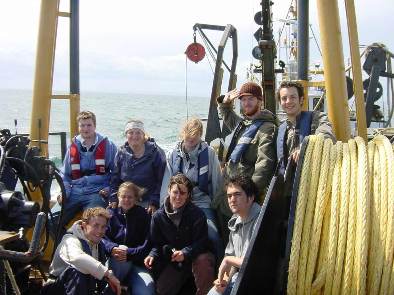
Figure 1 Members of group 11 aboard the Terschelling 

Introduction

Plymouth Sound, England, is located south of the confluences of the rivers Tamar and Lyhner and of the Tamar and Tavy, Devon. This web page summarises the preliminary findings from a group (fig. 1) of nine people, working in conjunction with eleven other groups, during an extended sampling effort carried out in Plymouth Sound and associated estuaries during June and July 2004. The aims of the investigation were to study the physical, chemical and biological characteristics of the estuary, and to draw appropriate conclusions about the processes governing these characteristics. Investigation by the groups as a whole extended from riverine end members near Calstock on the River Tamar out as far as E1, beyond Eddystone Rocks, offshore. 

The estuarine area investigated has a high diversity of habitats with a wide variety of flora and fauna. The northern shore of Plymouth Sound features a reef of submerged Devonian limestone. The Tamar Estuary is partially mixed and mesotidal, with a tidal range of 2.2-4.4m on neaps and 0.8-5.5m on springs relative to Chart Datum. There are extensive tidal mudflats and salt marshes. The mudflats are some of the largest in the South West, and provide habitats for an abundance of invertebrate species.  

Geology

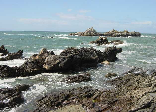
A brief study of the geological composition and fold geometry of an area of Heybrook Bay was undertaken on 24/06/2004. Strata layers that have been compressed and consequently folded are evident throughout Renney Rocks, which are located at the southern end of Heybrook Bay. Ancient plate movements and continental drift created sufficient stresses and pressures to create a series of fractures that radiate around 

a fault line. The compressive stress during formation of this geological feature resulted in a right lateral dextral fault with major displacement visible along the fault line. A conjugate set of fractures can be seen orientated at between 30º - 45º to the fault. Diagrams supporting this study    Fig 2. View of

are in the group log book.                                                                                                                                                                             Renney Rocks

A section of cliff face that runs parallel to the Renney Rocks area gives an indication of ancient deposition events, including periods of higher energy deposition. The cliff face has a reddish colour, indicating the presence of oxidised iron. This is characteristic of warm, humid climate periods at the time of deposition. The darker red band that is dominant throughout the cliff section demonstrates a period of highest incident radiation, evidently at the most recent climatic optimum (the Holocene) around 8000 years ago. This band consists of unsorted clasts imbedded within a coarse matrix and is representative of a "pulse" of energy, such as a landslide or mudslide during deposition. Throughout the strata within the cliff section the presence of small high-energy deposit layers indicate further, sudden "pulse" events,  adequate to form stratified sub layers. The angularity of the clasts that are visible along the cliff section indicate that weathering processes dominated by frost shattering were probably evident at that depositional period. Between 10000-18000 years ago the study area  was predominantly periglacial, which accounts for the occurrence of weathering processes such as freeze-thaw.   

return to top

RIBS

The aim of this fieldwork was to investigate the chemical and biological characteristics of the River Tamar from the riverine end member (0 salinity) found near Calstock (site 0: 50°29.616'N 004°11.684'W), to higher salinities near to the Tamar Bridge (site 30: 50°24.555'N 004°12.207'W) by using two small boats. Data collected on the day (02/07/04) were shared with group 10, who were working on the Bill Conway further down the estuary. An overlap in salinities sampled by the two groups was aimed for, in order to provide a continuum of measurements from the riverine end member to the saline end member. Surface water samples were analysed for concentration of nitrates, phosphates, silicate and chlorophyll. One further surface water sample per boat was taken using a Niskin bottle. This sample was analysed for concentration of dissolved oxygen analysis. At each sampling station, multi-parameter probes were used to measure salinity, temperature, dissolved 0₂, pH and depth in a vertical profile.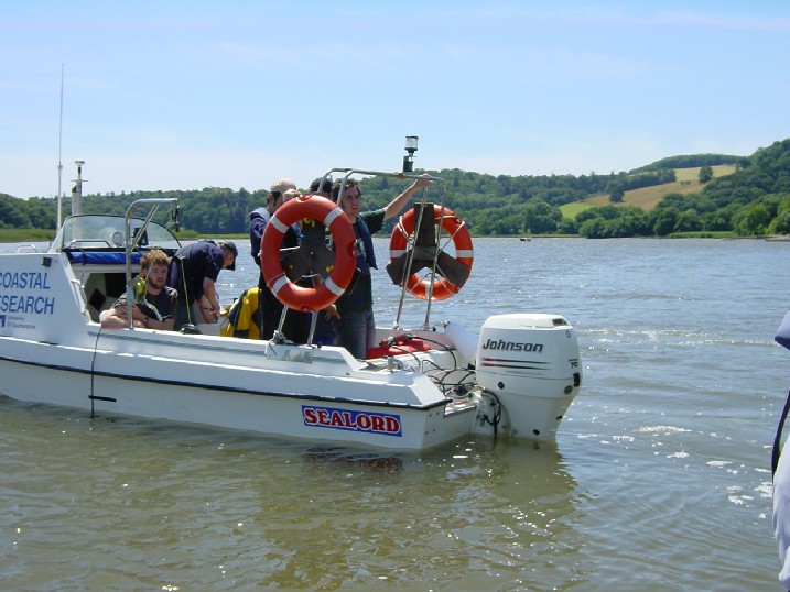 

The small boats (fig. 3) started up-river of Calstock at close to zero salinity. Samples were taken moving downriver at salinity intervals of 2, staggered between the two boats - each boat stopped at a station with every rise in salinity by 4. It was necessary to work in a direction moving downriver because of the 11:26 GMT high water at Calstock. Shallow depths at low water (0m above Chart Datum at low water) meant that 

starting at Calstock in this way allowed a greater salinity range to be sampled in the river. 

Three zooplankton tows at three separate salinity stations were carried out in order to measure abundance of zooplankton. The zooplankton nets were deployed by mooring them to a buoy at the chosen sites so that the river current was able to flow into the net itself. Eulerian style sampling was carried out, by reading a flowmeter attached to the zooplankton nets.

Figure 3 . Action on the boat 

Phytoplankton samples were obtained at the same sites as the zooplankton tows. Phytoplankton samples were preserved with iodide so that counts could later be performed in the laboratory. Both zooplankton and phytoplankton samples were used to give an indication of the relative abundance of these groups at different salinities in the river, although the small (3) number of samples taken precludes many specific conclusions from being made about biological processes.    

Water densities were calculated from temperature and salinity data from the multi-parameter probes used at on the small boats. This was done for every station sampled during the ribs boat work, between station 0 (GPS 50°29.616N, 004°11.680W, time 11.25GMT) and station 32 (GPS 50°23.978, 004°12.540, 14.57GMT).  These densities are displayed on the contour maps (figures 4 and 5).  Fig  4 shows density change with depth and salinity which, as would be expected from the equation of state, increases with increasing salinity.  There is little change in density with depth at constant salinity, demonstrating that at these shallow depths pressure is insufficient to have any significant effect on density.                                                    

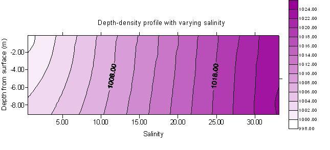
Figure 4. Density depth profile with varying salinity

Fig  5 shows the change in density with depth and station number. This provides a plot of the density stratification progressing downstream – a longitudinal cross section of the water body - showing that density increases with depth and site number (and therefore distance downstream).  This demonstrates the gradient of mixing of less dense fresh water from the head of the estuary – which lies closest to the surface - with more saline, denser water at the marine end of the estuary.  The saline water mixes with the overlying less dense fresh water, as can be seen in the density-depth-site number plot (fig 5).

Figure 5.   density depth profile from sites 0-32.

These data are limited by the fact that the data were taken at varying tidal states. The data would need to be taken simultaneously to produce an absolutely accurate plot of the density stratification of the water column.  These data do, however, show the trends that would be expected from the mixing mechanisms of an estuary.

Analysis of temperature vs. salinity depth profiles for sites 0-32.

Data from group 11 estuarine sampling effort using small boats can be found in the following directory:

group11\all_work\25-06rib\rib-data

For the ribs work, most site numbers correlate approximately to the surface salinity measured at that sampling station. 

At Calstock (at 0 surface salinity) the T/S profiles show fresh river water overlying colder saline water. There are a shallow thermocline and halocline at approx. 1m depth, and a temperature minimum of 15.6°C (at the bottom).

At sites 4, 6 & 8 there is a general increase in salinity with depth and a decrease in temperature with depth (as seen in all T/S profiles collected). The thermocline is still shallow at 1m depth. 

At sites 10, 12 & 14 the thermocline is still at 1m depth, the salinity still increases with depth and there is a steady decrease in temperature deeper than the 1m thermocline.

At sites 16 and 18 the thermocline is deeper (2m depth). The structure of the temperature remains roughly the same with approximately the same decrease in temperature with depth. 

At sites 22, 24 and 26 the water column is deeper and there is a further decrease in temperature with depth. The surface salinity increases from 20 to 23. 

At sites 30 & 32 (by the Tamar Bridge) the surface salinity reaches 30 and increases still with depth to 32.7. The structure of the temperature profile remains approximately the same.

Analysis of salinity vs. euphotic zone depth 

Euphotic zone depth was calculated as Secchi disk depth multiplied by 3. With increasing salinity, the euphotic zone depth was seen to increase. The magnitude of increase in euphotic zone depth between salinity intervals increased with proximity to the saline source.

As salinity increases, so too does the concentration of Na⁺ ions. These ions encourage suspended particulate matter (SPM) in the water column to coalesce, leading to the formation of larger colloidal  particles. These particles have a greater tendency to fall out of suspension to the seabed, therefore increasing light penetration and deepening the euphotic zone.  

Chemical Analysis.

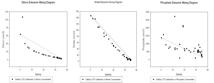
Fig 6: A (left), B (middle), C (right). Estuarine mixing diagrams for Silicate (A), Nitrate (B) and Phosphate (C) in the Tamar estuary.

Silicon  

Since all measured silicate concentrations (except one) fall below the theoretical dilution line (TDL),  non-conservative removal of silicon was observed (fig 6 A). One anomalous result was recorded at site 2  (at Calstock). This value was unusually high possibly due to the influence of a small tributary in close proximity to the site and up river. 

Nitrate 

Most data points occur in a moderately straight line slightly below the TDL (fig 6 B). This supports findings by Morris et al., (1981) who found an essentially conservative relationship between nitrate and salinity in the upper reaches of the Tamar Estuary. There appear to be no anomalous recordings for nitrate.

Phosphate (Data from Ribs only) 

Phosphate shows a non-conservative relationship in the estuary, with data points occurring both below the TDL (fig 6 C), indicating removal (lower salinities) and also above the TDL (higher salinities). At salinities above 25 there is an influx of phosphate into the estuary, shown by points above the TDL. This may be due to geographical features close to these sites. It is possible that the steep sides of the surrounding banks, large areas of agricultural land and increased surface run-off due to recent increased precipitation events, have elevated the phosphate concentration at these sites. Non-conservative and non-biological removal of phosphate could also be as a result of chemical precipitation of dissolved phosphate at lower salinities, as found in the Tamar Estuary by Morris et al., (1981).

Chlorophyll

The concentration of chlorophyll in the estuary is higher at low salinities (see fig 7), indicating that there is a decreasing abundance of phytoplankton heading seawards. This can be explained by increased grazing pressure by zooplankton further to seaward. Though species specific,  zooplankton tolerance of low salinities may be less than that of phytoplankton in many cases. This may allow phytoplankton to increase in abundance in the nutrient-rich waters further up the estuary in the absence of heavy grazing pressure by zooplankton. A Secchi depth of 19cm at the lowest salinity sampled (site 0) would allow enough light in the top 50cm (approx.) of the water column, to support primary production. Two zooplankton counts carried out in the estuary indicate that the abundance of zooplankton increases heading seawards, though more comprehensive studies are required to form definite conclusions. Higher primary production in the water column would be expected towards the seaward end of the estuary, because of increased euphotic depth. This would support a larger population of zooplankton at higher salinities. These zooplankton would be able to exploit a food source of phytoplankton to a limited extent up the estuary. 

The phytoplankton population seen at the marine end of the estuary exhibit features of the end of a spring bloom, being dominated by diatoms. As silicate is undergoing removal at the marine end of the estuary, diatoms        

may be becoming limited by silicate concentration. The Tamar Estuary has been shown to exhibit strong turbidity maximum in its low-salinity reaches (Grabemann et al., 1997). This results in a shallow euphotic depth at low salinities. Despite this, phytoplankton are able to exploit the nutrient-rich (figs 6 A, B, C) waters found at low salinities.

Fig 7. chlorophyll concentration vs salinity 

Dissolved Oxygen

Figure 8. A, B, C. Dissolved oxygen depth profiles for sites 0 (8A), 16 (8B) & 32 (8C).

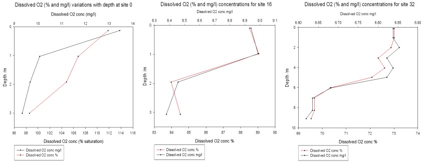
The dissolved oxygen depth profiles show in general a decrease in concentration with depth. The graphs above show dissolved oxygen depth profiles for close to zero salinity, mid-range salinity and high salinity (~32) values. Oxygen concentration in both % saturation and mg/l is observed as decreasing with increasing salinity.  The chemical reactions of photosynthesis evolve oxygen. Therefore higher concentrations of dissolved oxygen are to be expected in the surface waters where phytoplankton are actively photosynthesising.  The approximate euphotic depths calculated from the Secchi disk measurements at each station are 0.57m for station 0, 1.92m for station 16 and 4.8m for station 32.  At each station, dissolved oxygen concentrations decrease rapidly around and below the corresponding euphotic zone depth, showing that some of the oxygen present in the surface waters is likely to have been evolved by phytoplankton.  It should be noted that oxygen levels in surface waters will also be elevated by physical processes, e.g. diffusion and wave action, and the presence of dissolved oxygen is not entirely attributable to biological activity.

return to top

Offshore Boat Work

During the summer months the waters offshore from Plymouth are typically thermally stratified. The spatial and temporal extent of this thermocline determines the structure and functional properties of plankton communities. Vertical mixing is the main mechanism controlling the depth of the thermocline, and this process therefore has an effect on the chemical and physical properties of the water column and hence the distribution of phytoplankton and zooplankton in the water column. The aims of this practical were to understand how vertical mixing affects the vertical distribution of nutrients, dissolved oxygen and plankton in an offshore environment, and also an offshore-onshore transect. This was done using multiple techniques to gain a holistic view of the sampled environment.

Figure 9. Map showing sites sampled (water samples and CTD), ADCP transects and miniBAT transect. 

Six stations were sampled in the water off the coast of Plymouth. Figure 9 shows the position of CTD sites sampled, with ADCP transects indicated between them (note: latitude and longitude of these positions are shown in table 1).

Table 1. Positions and transect times for offshore ADCP.

Data from ADCP transects can be linked with those from the CTD dips (at the start and end of transects) and also zooplankton hauls, in order to provide a holistic interpretation. (Note: printouts for all CTD dips and ADCP transects for the offshore boat work are in the group logbook). CTD data were collected at all sites except site 6 because of technical difficulties with the equipment. 5 Niskin bottles, attached to the CTD frame, were used to obtain water samples at depths above and below the thermocline at each site. Water samples were analysed for nitrate, phosphate and chlorophyll concentration, and for dissolved oxygen (% saturation). Hauls of zooplankton (to sample a vertical profile of the water column) were taken at sites 1, 2, 3 and 6. Water samples for phytoplankton counts were taken at sites 3 and 5 and fixed in lugols iodine solution. Acoustic Doppler Current Profiler (ADCP) data were taken throughout the entire day. Data were taken using a towed undulating instrument, Minibat. These data were collected in an offshore-onshore transect between sites 3 and 4, travelling at reduced towing speed of approx. 4 knots. 

The CTD profile at site 1 (behind the breakwater - see table 2 for positions of all CTD sites) shows a thermocline and a halocline that are both steep and shallow (2-3m). There is a 0.5°C change in temperature across the thermocline and a change in salinity of approx. 1 across the halocline. Fluorescence readings are low at the surface, and higher beneath the thermocline. This could represent phytoplankton becoming trapped beneath the thermocline during a period of stormy weather (gales and heavy rain) five days previous to sampling, followed by some calmer weather during the day before. Strong winds would have mixed the ~12m deep water column, redistributing phytoplankton down throughout. During the ensuing calm weather, a large input of fresh river water could have contributed to the re-stratification of the water column, with the result that many phytoplankton could have remained trapped at depth.

Table 2. Positions of CTD dips

Moving offshore from site 1, the ADCP transect (fig. 10 data file in directory X:\group11\all_work\28_06off\off_data\off_raw\adcp) shows the inshore turbid waters as uniformly red on the left side of the image. As the transect moves offshore (looking from left to right) there is a layer of backscatter that is shallow (just below the surface) to start with; then deepening to approx. 8m. This scattering layer is probably the chlorophyll maximum. The chlorophyll maximum grows deeper moving offshore because the water column is stabilised by solar heating during the summer, producing a deeper thermocline. Phytoplankton generally grow optimally at the depth of the thermocline because this is usually the depth where there is optimum availability of both light and nutrients. Offshore waters off Plymouth have been shown to have maximum chlorophyll levels at depths below 10m and within the seasonal thermocline (Holligan et al., 1983). This is supported by the CTD profile from site 2 (L4). The profile (printout in logbook) shows a deep and gradual thermocline extending from approx. 4m to 40m depth. Within the thermocline fluorescence is highest (1.5-1.8µg/l) indicating that the chlorophyll maximum is spread over the extent of the thermocline. Water samples taken during this profile confirm this. On this transect (between sites 1 and 2) the ADCP has also picked up a signal which probably corresponds to fish. This is shown by some pulses of high return (shown by red stripes). The ADCP transect (fig. 10) finishes at site 2, where two zooplankton hauls were carried out, from above and below the thermocline. Counts from the zooplankton haul from below the thermocline (sample 2c. 50m to 38m figure 16, abundance of zooplankton) give a number of 6.34*10⁶m^-3. Counts from the zooplankton haul from 38m to the surface (sample 2a) give a number of 1.7*10⁷m^-3. These data therefore indicate that the abundance of zooplankton is greatest within the thermocline at site 2. Since this shallower zooplankton haul would have sampled through the scattering layer (green, fig. 10) it appears that there is a good correlation between the depth of the chlorophyll maximum, depth of maximum zooplankton abundance and depth of scattered layer as shown by the ADCP.

Figure 10 (left) ADCP transect between sites 1 and 2 showing the deepening scattered layer .                      Figure 11 (right) ADCP Transect between sites 2 and 3 showing the observed front

The CTD profile at site 2 shows a thermocline that is less steep, extending over a greater depth. Note: the thermocline at this site (site 2) represents a change in temperature of approx. 2 °C, from 14 °C down to 12 °C. At site 1 the change in temperature across the thermocline was only approx 0.5 °C. Since site 1 is further inshore and behind the breakwater, the warmer river water would have a greater influence here. Offshore, at site 2, there is colder (12 °C) water at depth. The river water from the estuary does not have a direct effect. Surface water is warmed by solar heating and the water column hence becomes stratified. The effect is seen over a greater distance vertically: the thermocline extends from near the surface to approx 40m depth, and is gradual.

The ADCP data from the transect between sites 2 and 3 show a frontal system (fig. 10). This can be seen in the middle of the image as a thick scattered layer from ~14m depth extending up to near the surface (green) meeting a layer with low scattering (blue) this second layer overlies the scattered layer of the first water mass. The velocity magnitude plot does not show any specific anomalies, and it is likely that the front is being passively moved by currents in the water.

The miniBAT was towed from just after the start of the transect from site 3 (start GPS 50°18.098N 004°21.186W, time 12.55GMT) for part of the transect distance to site 4, stopping at 50°20.778N 004°21.186W, 13.33GMT. The depth-time profiles for several parameters are displayed below, dark green representing the higher values and blue the lower values in each case.  The path of the miniBAT through the water is also marked on each plot with a light green track plot.  The path is spread well throughout the body of water sampled, so the data can be expected to be accurate, perhaps with the exception of the data below 15m depth for time 0.00-20.00 (arbitrary time units) for which there are no real data.

The transmittance plot shows decreased transmittance towards the end of the tow, between the surface and 8m depth. This is not coupled with an increase in fluorescence, indicating that the increased transmittance is due to the presence of suspended particulate matter rather than biological activity.  Being closer to the shoreline, it is possible to suggest that this is caused in turn by an increase in wave action and mixing processes in shallower water due to shear stress with the sea bed. Wave action would also increase the amount of oxygen in an area; this is supported in the dissolved oxygen data, with an increase in the amount of oxygen in the same area. However, it should be noted that the column of very low values just before this section is present throughout the water column and is likely to represent a failure in the instrumentation resulting in erroneous data.

Figure 12.   miniBAT profiles from offshore boat work 

Figure 13. comparisons between miniBAT and ADCP data

Between site 3 (50°17.823’N, 004°23.950’W, 12:40 GMT) and site 4 (50º 20.778'N, 004º 21.186'W, 13:33 GMT) the CTD data shows the chlorophyll maximum being pushed upwards in the water column from a depth of 19m at site 3 to approximately 12m at site 4, despite the presence of an obvious thermocline to hold the phytoplankton in place at site 4 indicating that the phytoplankton are being pushed onshore.  This could be occurring due to the south westerly winds in the area for at least a week prior to sampling, or due to the river plumes from the estuary encouraging onshore currents in Whitsand bay.  The data displays how the physical mixing processes in the shallowing water push the phytoplankton and therefore the chlorophyll maximum closer to the surface.

Salinity decreases along the tow, moving inshore. There is little or no vertical stratification of salinity along the tow. Slightly lower salinity represents the present, but limited, influence of the river plume from the estuary mouth.

Temperature shows vertical stratification, and very slight horizontal stratification, maximum temperatures found at the surface and inshore. The thermocline is at approximately 5m depth at the beginning of the tow, and finishes at approximately 10m.

All files relating to the minibat work, including grid files etc. can be found under group11\All work\28-06-04-off\Off_data\off_proc\minibat

Analysis of water samples - offshore work

A brief description for the procedure followed for measuring nitrate concentration is given in the directory:

group11\All work\28-06-04-off\Off data\off proc\chemanly

Profile shapes for chlorophyll concentration are approximately mirrored by those for silicon concentration (fig. 14). This indicates that the concentrations of chlorophyll and silicate could be linked by a biological process in the water column (primary production). As phytoplankton primary production takes place, the nutrients nitrate, phosphate (and silicate for diatoms) are absorbed. Hence, the water sample concentrations for these nutrients are seen to be low where chlorophyll concentration is high. 

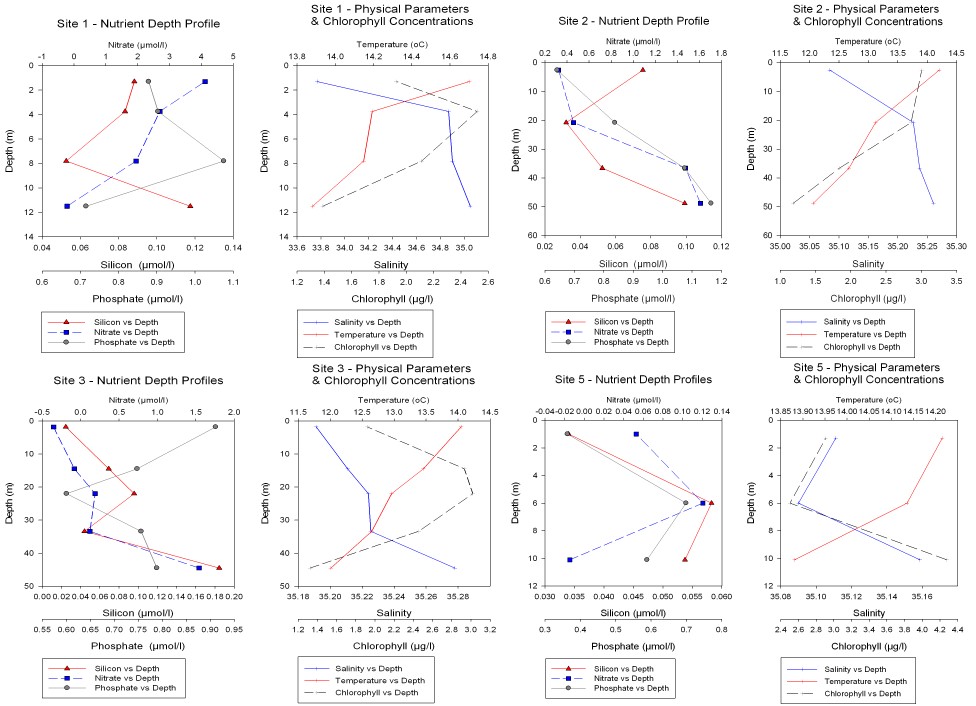
Figure 14. Nutrient concentration vs depth for stations 1,2,3 & 5 

Chemical Analysis

Chlorophyll

Site 1 (behind breakwater: all lat. and long. positions of sites are given in table 2). There is a good correlation between depth of chlorophyll maximum and depth of nitrate and silicate minima at site 1 (behind the breakwater. Position of site in table 2). 

Sites 2 and 3 (offshore) both show an opposing trend of high chlorophyll concentration at the same depth as low concentrations of silicate and nitrate (fig. 14). From data collected with the ADCP, site 2 (L4) appears to be located on a frontal system (fig. 11. Data file oadcp11003r.000 in the directory group11\all_work\28_06off\off_data\off_raw\adcp). The mixing conditions that produce frontal systems determine the availability of light and nutrients necessary for phytoplankton growth. (Pingree, 1975). This in turn has an effect on the depth of the chlorophyll maximum, and the concentration of chlorophyll present. At site 2 the chlorophyll maximum appears to be close to the surface. Surface concentration of chlorophyll at this site is high (3µg/l). The chlorophyll maximum has been pushed down from the surface waters to a depth of 20 m with concentrations of 3µg/l.

Site 5 (inshore). From the CTD data the temperature and salinity profiles show that the water column is well mixed and that the water depth is deeper than the thermocline depth. The chlorophyll maximum has been pushed down to the bottom of the profile. The absolute highest concentration of chlorophyll were recorded at the bottom of the site 5 profile at 10m depth of 4.3µg/l. Site 5 was quite far inshore (table 2), and the presence of the chlorophyll maximum at depth could represent phytoplankton being driven onshore from deeper offshore thermoclines by currents and stormy weather.                   

Nitrate/nitrite  

Brief analysis is given for sites where sufficient samples have been taken in order to provide a sensible interpretation

Site1 (behind breakwater). Nitrate and nitrite concentrations decrease with depth. However, concentrations of these nutrients do not increase as the Silicon levels do at 8m depth. This indicates that there is no bottom water nitrate and nitrite input. Since site 1 is landward of the breakwater, high nitrate and nitrite levels in surface waters may represent fresh water inputs, which are enriched by agricultural runoff. At site 1 we see the absolute highest concentrations of nitrate and nitrite from all the sites at 4µm/l at the surface.

Site 2 (offshore). Nitrate concentration (includes nitrite) increases rapidly below 30m up to 1.7µmol/l. This indicates that there is little or no mixing between the nutrient-rich bottom waters and the phytoplankton-rich surface waters.   

Site 5 (inshore).   A good correlation of decreasing nutrient levels with increasing chlorophyll concentration exists, with the chlorophyll maximum and nutrient minimum at 6m depth.

Silicon

Site 1 (behind breakwater). The positioning of site 1 (see chart) behind the breakwater in the Sound has produced the expected results for chlorophyll with Silicon (fig. 14 - Station 1). These results are: a Silicon minimum corresponding to the depth of the chlorophyll maximum. Below the chlorophyll maximum concentration of Silicon increases.

Site 2 (offshore). Surface Silicon levels at site 2 are slightly higher than expected; this may be due to the end of the spring bloom of diatoms meaning that this nutrient is no longer scavenged in surface waters. Below the thermocline (see also CTD data in the directory: group11\all_work\28_06off\off_data\off_proc\ctdproc) the nutrient levels are much higher than the surface concentrations.

Site 3 (offshore). The absolute highest concentrations of Silicon were found in the deep (~45m) waters at this site, with values of 0.18µm/l.

Phosphate

Site 1 (behind breakwater). At this sampling station the phosphate concentrations do not follow the trend of silicon and nitrate. This anomaly may be due to the large fresh water input following a period of heavy rain, and also possibly the influence of the breakwater in close proximity. 

Site 2 (offshore). At this site the highest (1.18µm/l) values of phosphate for all offshore sampling sites from the day were recorded, below the thermocline at around 50m depth. 

Site 3 (offshore). the phosphate levels are high at the surface and decrease with depth towards the chlorophyll maximum (around 20m).

Dissolved oxygen

Site 1 (behind breakwater). The dissolved oxygen against salinity plot shows that the water column is well mixed. Dissolved oxygen shows a decreasing trend with increasing salinity up to 34.3 and then fluctuates with increasing salinity.

Site 2 (offshore). Dissolved oxygen decreases from 86% saturation to 73% saturation with increasing salinity. This is similar to site 3 (also offshore), at which the saturation % decreases from 87% to 73%.

Biological Analysis

At all sites the dominant species are heterotrophic dinoflagellates, contributing to more than 70% of the population in all samples except for site 1 (behind the breakwater). At site 1, there are approximately equal numbers of copepods and heterotrophic dinoflagellates. This could be due to this site's position at the mouth of the estuary and hence higher phytoplankton abundance.

Sites 1 and 5 (both near shore sites) contain the highest species diversity. This may be because of optimum physical conditions and nutrient availability. From the data a dinoflagellate bloom was observed at the inshore sites. These blooms are very important to the system due to their contribution to annual primary production (Holligan et al. 1981). This compliments the high zooplankton diversity seen at sites 1 and 5. Ctenophores and fish larvae were only seen at site 1, again suggesting these sites' high productivity.

 Site 3 shows a wide marine diversity, having large abundances of echinoderms, siphonophores and medusae (which the other sites were lacking or had much less of). Site 2, the L4 site, had comparatively low species diversity, having dinoflagellates as 80% of the community structure; a front was discovered in the ADCP data between sites 2 and 3. Fronts are significant in determining distributions in phytoplankton (Pingree et al. 1975). 

Figure 15. Zooplankton composition from offshore samples                                                            

Table 3. Positions and depths of zooplankton nets (200µm mesh). Offshore boat work.

Figure 16. Abundance of zooplankton at the sites sampled during the offshore work. Note: sample 3c is of a horizontal tow at approx 2m depth.

return to top

Estuarine Boat Trip

This procedure aimed to develop an understanding of how the Tamar Estuary acts as a transition zone between the freshwater input and the coastal sea. Eleven stations were sampled on 02/07/04, shown in Figure 17, in conjunction with the ribs group (group 10) in order to produce a holistic view of the estuary. ADCP transects were used to distinguish velocity magnitude, shear direction and backscatter. CTD profiles were used to observe the features of the taken transect. Four Niskin bottles, attached to a CTD rosette, were used to gain water samples for nutrient, chlorophyll and dissolved oxygen analysis from varying depths. Plankton nets were towed at two sites, the most marine being site1 and the most freshwater, site 11, for direct comparison. A Secchi disc was used to determine the euphotic depth at most sites. Phytoplankton samples were taken from the surface and preserved in Lugols iodine solution for laboratory analysis.

Figure 17. Sites sampled during estuarine boat work on Bill Conway

Temperature and salinity depth profiles

Site 1 – In the middle of the Sound, the water column is fairly well mixed, with very little difference between the surface and bottom water temperature and salinity.

Site 2 – On the East of the sound, there is stratification in the surface waters, with a thermocline at 6m depth.

Site 3 – West of Sound. Still fairly well mixed with a thermocline at 6m.

Site 4  - Cattewater – Gradual decrease in temperature from the surface (15.3 °C) to 14. 8 °C at 6m. Surface salinity is lower at 32.6 compared to previous sites, and increases with depth i.e. there is a small salt wedge.

Site 5 & 6 – The Narrows – There is very little change in temperature and salinity with depth. Therefore, a well mixed water column.

Site 7 – Tamar Bridge – Less saline water with maximum salinity at the surface (31.0) There is a shallow thermocline at 2m but the water column is still fairly well mixed, with a change of only half a degree. Surface temperature is 16.9 °C. This is two degrees warmer than the more marine sites.

Site 8 – The observed front by the Tamar Bridge. It is more saline at the surface and increases with depth to 33.5. There is a relatively large change in temperature between warm surface waters and colder bottom waters.

Site 9 – The observed front by the Lynher – This profile shows a split thermocline with well mixed bottom waters.

Site 10 – Mouth of Lynher – More saline and colder at the bottom. Temperature at the surface is 16.35 °C

Site 11 – St. John’s Lake – There is a salt protusion at 4m depth of 34.36 that decreases rapidly to 14.84 °C.

ADCP ANALYSIS- Bill Conway, 2^nd July 2004

Table 4. Analysis of estuarine ADCP data

Secchi disc analysis

Site 1 has the greatest euphotic zone at 12.18m because it is the most marine environment and has the least suspended sediment, due to an increased amount of Na⁺ ions. These tend to cause sediment particles in the water column to coagulate; falling to the bottom.

At site 2 colour filters were used, to show which wavelengths of light were attenuated first. The first wavelength to be completely absorbed at 1.21m was red, followed by green at 1.4m then blue at 1.88m. This indicates a high phytoplankton abundance at this site, as a large amount of green light would be absorbed due to the high chlorophyll concentration.

Nutrient concentrations with depth profile analysis.    

Figure 18. Nutrient and chlorophyll profiles from 02/07/04.

Figure 19. Estuarine mixing diagrams from boat work carried out on 02/07/04

Chlorophyll

Site 1. By the breakwater. The chlorophyll concentrations in this profile are the lowest of this set of profiles from Plymouth sound to the Tamar bridge suggesting that either the physical conditions and availability of nutrients at this site (the most seaward profile) may be limiting phytoplankton growth, or the grazing pressure from seawater zooplankton may be limiting the abundance. Without knowing the amount of primary production occurring in this location we can not determine which situation is the most representative.

Site 2. Towards the east of the Sound. The maximum chlorophyll concentration occurs at the top of this profile in the surface waters of 13.2μg/l.

Site 4. This profile shows opposing chlorophyll and nutrient concentrations, as phytoplankton abundance increases with depth.

Site 5. The Narrows. This profile was taken at slack water in a region where there is high velocity flow over much of the tidal cycle. The nutrient and chlorophyll depth profiles show extreme mixing, with fluctuating peaks of high and low concentrations.

Site 7. By the Tamar bridge. The surface concentrations of chlorophyll, nitrate and silica are all very high (12μg/l, 22μmol/l and 0.048μmol/l respectively) and decrease with depth.

Site 10. Mouth of the river Lynher.  At this site fresh water anomalies were observed from the boat and the definition between the fresh input and the rest of the water mass could clearly be seen as a foamy, bubbly film which was caught in the convergence between water masses.(See adjacent photo.)

Elevated silicate concentrations may represent the presence of a diatom population around this front or simply high surface nutrient concentration. The chlorophyll concentrations at this and other upstream sites may be elevated due to there being less fresh water zooplankton than saltwater zooplankton at the sites towards the seaward end of the estuary. The maximum chlorophyll abundances will appear closer to the surface the further up the estuary as high suspended sediment load in the water column reduces the euphotic depth.

Nitrate/nitrite

Site 1- In the middle of the Sound we see the lowest nitrite and nitrate concentrations of only 0.93 μmol/l in the surface waters, peaking in this depth profile at around 8m with 1.08μmol/l and almost depleted in the bottom waters. This indicates that the supply of nitrate and nitrite to Plymouth sound is not from the saline bottom waters but from the fresher riverine waters.

Site 2 The nutrient concentrations are still relatively low and deplete towards the bottom of the profile with a peak at 4m depth.

Site 4 the nitrate concentrations decrease with depth.  The surface nitrite and nitrate concentration at this site is elevated relative to other sites with a maximum of 14.5μmol/l. This elevation suggests a localised input of nitrogen to the estuary. Looking at the charts this location, at the mouth of the dredged Cattewater river, is a heavily polluted input into the sound with silos and other sewage pipes discharging organic and inorganic nitrogen forms. There is an Esso wharf also located by the site.

Site 5 - Nitrate concentration generally decreases with depth.

Site 7 By the Tamar bridge. The surface concentrations of chlorophyll, nitrate and silica are all very high (12μg/l, 22μmol/l and 0.048μmol/l respectively) and decrease with depth. At this site inputs upstream may be affecting the concentrations measured. On the charts, sluices and silos as well as other pipes all discharge into the river. There is also agricultural land further upstream, and runoff from these lands (pesticides. herbicides and excretory products) may also be contributing.

Site 10 The water profiles show high surface nitrate concentration (10μmol/l) which decreases with depth (however are still relatively high at the bottom of the profile at 8 μmol/l).

Silicon

Site 1. The distribution of Silicon and chlorophyll follows the same pattern as nitrate, with peaks of 0.0352μmol/l and 2.85μg/l respectively at 8m depth.

Site 2. The nutrient concentrations are still relatively low and deplete towards the bottom of the profile, with a peak at 4m depth.

Site 4. The silicon concentrations decrease with depth.

Site 5. Chlorophyll and silica concentrations peak at 10 m depth.

Site 7. By the Tamar bridge. The surface concentrations of chlorophyll, nitrate and silica are all very high (12μg/l, 22μmol/l and 0.048μmol/l respectively) and decrease with depth.

Site 10. Surface chlorophyll and silica concentrations are also high (10.5μg/l and 0.0397μmol/l) and follow the same trend as nitrate of decreasing concentration with depth.

Phosphate.

Site 1. The lowest estuarine phosphate levels were observed here, being 0.62μmol/l at the surface and increasing in concentration with depth.

Site 2. Very low phosphate concentration at the surface, increasing with depth.

Site 5. At the narrows the water column is well mixed, with high concentrations of around 1.5μmol/l.

Site 7. High surface concentrations (1.35μmol/l) increasing with depth to 1.43μmol/l.

Site 10 (Tamar Bridge). The highest estuarine concentrations were measured here, being 1.6μmol/l in the surface waters. The elevated phosphate levels at these upstream sites are possibly due to agricultural runoff (organo-phosphates from fertilisers). The general trend of estuarine phosphate was found to be that surface concentrations increase the further upstream.

Dissolved oxygen

return to top

Geophysics boat practical 05/07/04

The aim of the geophysical practical was to conduct a detailed seabed survey of the region to the south of Plymouth breakwater. The survey included acquisition of sidescan sonar and bathymetric data and retrieval of grab samples. The sidescan sonar, towed behind the catamaran NatWest 2, is used to observe the bathymetry of the seabed. The transmitter within the fish is towed behind the vessel. Transmissions are reflected from the seabed and receivers in the fish relay the information to onboard computers, and on to a printer chart where immediate analysis can be made. From this and the global positioning data (GPS) a plot could be made back at the lab, bearing in mind the layback which is the distance the fish is away from the onboard GPS due to the fact that the GPS on the ship is approximately 5m to the stern plus the distance the fish is away from the vessel. It is an image of this plot that is below, on top of the plot is some images of features that will aid to the understanding of the sidescan data.

From analysing the data it is possible to calculate, using Pythagoras theorem, the distance away from the centre of the trap objects are and also the height of objects protruding from the seabed.

 Multiple sites were surveyed to try and find some interesting data, but due to the divers over the James Egan Layne it was not possible to get as much information as desired. The analysis below refers to site 3 of the sidescan sonar sites.

Fig. 20  All sidescan survey sites                                      Fig. 21 sidescan survey site 3                      Fig. 22  sidescan sonar plot                          Fig. 23 vertical rock strata

(group11\all_work\05-07gp\pics\geopic)

Analysis

Summary

The data collected from 25/06/04 (ribs) 28/06/04 (offshore on Terschelling) and 02/07/04 (Bill Conway) indicates that the Tamar Estuary is a partially mixed. Throughout the estuary, silicon is removed and nitrate is conserved. Phosphate is probably non-biologically removed at low salinities. This nutrient is added at high salinities. These nutrients are found in higher concentrations upstream towards Calstock as farmland runoff and small tributaries provide the estuary with a source of silicate, nitrate, nitrite and phosphate.

From the samples of phytoplankton and zooplankton collected from various parts of the estuary and offshore, we concluded that the tail-end of a dinoflagellate bloom had been sampled offshore. There is a higher species diversity of zooplankton in the marine environment than in the estuary. High quantities of freshwater phytoplankton were collected. Chlorophyll data and plots complement these findings.

CTD profiles show the development of a seasonal thermocline offshore. The riverine influence in terms of freshwater is not easily seen beyond the breakwater at the southern end of Plymouth Sound. In the estuary, fresh water flows seawards overlying the more saline. Since the estuary is partially mixed, the tidal influence can be seen up the estuary to Calstock, where 0 salinity fresh water overlies water of salinity ~7.5.

 An appreciation of the use of sidescan sonar in geophysical seabed surveying, was also achieved.

Return to top

References

Grabemann, I., Uncles, R. J., Krause, G. and Stephens, J. A. (1997) Behaviour of Turbidity Maxima in the Tamar (U.K.) and Weser (F.R.G.) Estuaries. Estuarine, Coastal and Shelf Science 45:235-246.

Holligan, P. M., Viollier, M., Dupouy, C. and Aiken, J. (1983) Satellite studies on the distributions of chlorophyll and dinoflagellate blooms in the western English Channel. Continental Shelf Research 2(Nos 2/3):81-96.

Morris, A. W., Bale, A. J. and Howland, R. J. (1981) Nutrient Distributions in an Estuary: Evidence of Chemical Precipitation of dissolved Silicate and Phosphate. Estuarine, Coastal and Shelf Science 12:205-216.

Pingree, R. D. (1975) The advance and retreat of the thermocline on the continental shelf. J. Mar. Biol. Ass. UK 55: 965-974.

Pingree, R. D., Pugh, P. R., Holligan, P. M. and Forster, G. R. (1975) Summer phytoplankton blooms and red tides along tidal fronts in the approaches to the English Channel. Nature 258:672-677.