Tim Barnes, Jo Dagnan, Bart De Baere, James Heywood, Lisa Jenkins, Becky Landers, Liam Sheena, Matt Suchley, Jenny van Santen  

CONTENTS

Introduction

Estuarine Boat

Chemical

Physical

Biological

Geophysics Boat

Geofield

Geophysics

RIB

Chemical

Physical

Biological

Offshore Boat

Chemical

Physical

Biological

Conclusions

References

HOME

INTRODUCTION

The study of oceanography is of vital importance to the progress and understanding of the dynamic environment that is the world’s oceans. Oceanography is sub divided into three individual but co-dependent disciplines, physical, chemical and biological. Estuaries are ubiquitous to our oceans boundaries and have been of great importance throughout time. Plymouth Sound and the Tamar estuary are situated on the south-west coast of the United Kingdom and are used for many purposes by naval and commercial vessels. The entire length of the Tamar estuary is less than four kilometers. The estuary is mainly fed by the Tamar river, which flows into the Hamoaze, where it is joined by the Lynher and St Germans before entering Plymouth Sound. The river Plym is also an important tributary of the estuary and is over 30 kilometers in length. Plymouth Sound enters the English Channel to the south and is therefore subject to tide and wave action. These physical conditions along with anthropogenic factors define the specific parameters which develop along the Tamar Estuary.

As a group of Southampton University students, we undertook a two week intensive field based, integrated study of the Tamar estuary and coastal waters. Four boat based practicals were scheduled for each group,  with sampling ranging between offshore to locations in the upper estuary. A variety of vessels were used to sample the water column ranging from the Terschelling, a 120ft, 300 tonne research vessel, to two small ribs for sampling in the upper estuary. Furthermore, the labs of Plymouth University were used to analyze the data collected, in order to produce individual reports and a group webpage and presentation of our finding.                                                                                                                                                               

1. ESTUARINE BOAT TRIP (X:\group10\processed data\Estuarine boat)

Date 25/06/04. Location: sampling within the Tamar estuary. Weather: large cumulus clouds however sunny - cirrus clouds noted further seawards. Tides:  High Tide 10:40GMT (11:40BST) Low Tide 17:40GMT (18:40BST) Research Vessel: Bill Conway

The aim of this boat trip was to obtain an integrated overview of the physical, chemical and biological processes within the estuarine waters.  The RV Bill Conway, Figure 2, equipped with an ADCP, CTD, rosette with 4 Niskin bottles, Secchi disk, zooplankton net and a pumped water supply was used to carry out a series of experiments.

1.1 CHEMICAL INTERPRETATION  (X:\group10\processed data\Estuarine boat)

Mixing profiles (e.g. silica)

Surface water samples were collected using ribs (group11) and the Bill Conway (group 10) on 26.06.04 in the Plymouth estuary. In terms of silica, non-conservative mixing appears to take place along the salinity gradient. Removal is taking place. Similar to the silica profile, nitrate removal has taken place along the salinity gradient, but to a lesser extent than silica. The removal of silica in low salinities (0-10) may be non-biological due to high turbidity and its inclusion into sediments. Nitrate removal can be correlated with nutrient uptake due to phytoplankton production (Morris, 1980). In terms of phosphate, a more scattered mixing profile has been obtained. Potentially, a removal in the region of 0-15 PSU and an addition in the region of 15-35 PSU is taking place. In the lower region  of the estuary, phosphate inputs could be attributed to runoff from arable land, and sewage inputs from urban area of Plymouth.

1.2. PHYSICAL INTERPRETATION

ADCP (X:\group10\processed data\Estuarine boat\adcp)

4 ADCP transects were carried out in the Tamar Estuary. Start and stop positions are shown in map 1(Plymouth Sound), 2 (The Narrows & scum line) and 3 (Tamar Bridge). Transect 8, carried out North of the Tamar Bridge was particularly interesting due a well defined thermocline and halocline discovered at a depth of 6m. The average backscatter calculated from the ADCP North of the Tamar Bridge shows a 'light blue finger' either due to a zooplankton column or the physical characteristics i.e. the thermocline and halocline found at 6m. These characteristics are really very unusual for an estuary and can not be explained fully without further investigation. However, it is hypothesised that the light blue finger could be directly influenced by the physical features found in the water column. Weather conditions could also have influenced the stratification observed throughout the water column. 

CTD - WATER COLUMN STRUCTURE (X:\group10\processed data\Estuarine boat\CTD)

Out of the 13 CTD profiles recorded, CDT 4 on transect Ramscliffe Pt.-Fort Pickcombes, CDT 6 in 'The Narrows' and CTD 11 upstream the Tamar Bridge will be discussed. Salinity and temperature profiles of the CTD stations are shown by clicking on the following links: CTD4, CTD6 and CTD 11. 

Vertical stratification increases higher up the estuary with a stronger thermocline. The deeper less pronounced thermocline in ‘The Narrows’ shows that vertical mixing between the fresher river input water and the deeper more saline water has taken place.  Salt water from the lower layer is entrained into the upper less saline water.  The water column is deeper at the Narrows compared to up-stream of the Tamar Bridge. Heading seaward down the estuary, the surface salinity increases as vertical mixing between the saline bottom water and the less dense river input water takes place. The thermocline and halocline becomes progressively weaker the more seaward the location with more effective mixing of the water column by winds and tide. The vertical profile of the water column becomes increasingly homogeneous up the estuary. It has to mentioned that the salinity and temperature gradient with depth is limited at all locations, so it can be concluded that the estuary is fairly well mixed.  Weather conditions prior to our sampling, could be a contributing factor. 

Transmission and fluorometry  profiles at stations CDT 4, CTD 6 and CTD11 are significantly different. Generally, values increase with depth and most significantly at the depths corresponding to those of the thermocline. Transmission and fluorometry are politely correlated with depth at Station CTD 11, but not at the other two stations. 

1.3. BIOLOGICAL INTERPRETATION

NUTRIENTS RESULTS (X:\group10\processed data\Estuarine boat\nutrients)

Water samples were collected at three locations at depths decided after looking at initial CTD profiles of the water column.

 Depth profiles of Silica and Nitrite were obtained at CTD Stations 4, 6 and 11 with the comparison of results from CTD Stations 4 and 11 being the most notable:

Station CTD 4: Nitrate concentrations decrease with depth from 5.75 µmol/L near to the surface to 4.5 µmol/L at 10m depth. Silica concentrations are highest near the surface and at depth. A distinct minimum is found at 7 m. Phosphate concentrations show a negative correlation with those of silicate. A peak is visible at 7 m.

Station CTD 11: The nutrient profiles are significantly different from the other two stations. The nitrate, silica and phosphate concentration profiles show a positive correlation.  The highest nitrite concentrations are at the surface (10.59µmol/L) and decrease considerably with depth, to 4.32 µmol/L at 9m depth. Phosphate concentrations are also elevated at the surface (600 µmol/L) and decrease to a minimum at 4m depth. Below 4m, concentrations increase again with depth. 

NUTRIENTS INTERPRETATION

N, P and Si are introduced naturally into coastal waters through atmospheric deposition, fresh water runoff and ground water seepage, through soil leaching and channel flow via rivers. Elevated concentrations of nitrate, phosphate and silicon are found in surface waters at the station highest up the estuary.  This could indicate an input of nutrients from river water draining the surrounding area. Coastal waters experience elevated concentrations of nitrogen and phosphorus due to anthropogenic inputs from urban and rural wastewater, wastewater and soil erosion. This would appear to be the case in the Tamar estuary. Silica is carried into the sea from water which has run-off areas composed of siliceous bedrocks. The dissolution of these rocks increases the silicon concentration within the run-off water.

DISSOLVED OXYGEN (X:\group10\processed data\Estuarine boat\Dissolved oxypros)

The lowest % saturations are at the most seaward station, CTD 4 (77.6), and at depth. The highest % saturations are in the near surface waters at stations 4 and 6 (81.1) and show values that decrease with depth. Higher up the estuary, the highest % saturation (81.2) is found at 9m.

The plots of chlorophyll  and nitrate concentration against salinity show a positive correlation, with the highest chlorophyll concentrations being found higher up the estuary, in the region of lower salinities (between 0 and 10 PSU).  The highest nitrate concentrations are also found in this region (values greater than 100µg/L). The growth of phytoplankton cells are not nitrate limited.  The region higher up the estuary also show higher, dissolved oxygen saturations, this could correlate to higher phytoplankton production in this region.   

2. GEOPHYSICS BOAT TRIP (X:\group10\processed data\Geology)

2.1. GEOFIELD EXCURSION

Date: 24/06/04 Location: Renney Point, Heybrook Bay Weather: wind Force 4/5, rain with sunny intervals. Tides: HIGH 09:38GMT (4.5m) LOW 15:35GMT (1.8m). Research Vessel: NATWEST.

At Renney Point, a sandstone outcrop is exposed in the cliff section. A distinct antiform fold extends southwards, plunging at 08º and with a strike of 232º. Bedding planes have dips between 30 and 63º and strikes between 55 and 172º to the west of the fold. A right lateral (dextral) fault with an orientation of 122º displaces the fold hinge by 8m. Overlying this formation there is a 4m terrestrial, post glacial to Holocene (from 18 000 BP and over the last 10 000 years) deposit. Sea level rise occurred in the area over this period. Looking at the image of this layer, the red colour can be explained by the oxidation of Fe. Deposits from short lived events are preserved in this section. Large, poorly sorted, clasts are situated at the foot of this section, deposited by a rock fall possibly due to cracking of rocks due freeze thaw, in post glacial conditions. A smaller grained sand and mud layer overlies these clasts which were probably deposited by fluvial conditions. A large 1m section overlies this layer, indicating possible catastrophic slope failure.  Angular clasts show a debris flow deposit.  Flow shearing is visible above this debris flow layer, and we observe a lighter sediment colour.  More sorted sediment is visible higher up the section with small clasts seen in a sand matrix which reduce in size towards the top of the section.  Shell fragments can be seen 50cm from in top of the cliff section.

2.2. GEOPHYSICS BOAT (X:\group10\processed data\Geology)

Date: 28/06/04 Location: various locations along the Tamar estuary.  Weather: sunny am, overcast pm. Tides: HIGH 13:20GMT. 

INTRODUCTION

The Natwest was equipped with GPS, the Van Veen grab and sidescan sonar.

Side scan sonar can be used to complete geological surveys and aid in artefact location i.e. ship wrecks. The equipment comprises of a fish (see figure 4) which produces acoustic signals at 100 and 500 Hz. The higher frequency is used to travel a greater distance but has less resolution.  The signal is then returned to the receiver with varying strength due to the presence of differing orientation of structures and sediment density. Hard sediments are shown up on the side scan graphs as dark, lighter images indicate soft sediments. The shadows cast by the relief of the estuarine bed are illustrated by white areas behind dark protrusions Side scan sonar releases the acoustic signals which at maximum efficiency can relay information up to 75m on each side. Problems with the side scan include: Layback- The fish is towed at a distance at the stern of the boat and the GPS recorded is from a fixed point in the vessel not at the exact point of the fish. This distance is lay back. However the GPS is accurate to +-10 m so was sufficient for this instance. Time Vary Gain TVG is another problem faced by this instrument. As the pulse of acoustic energy propagates through the water it is attenuated. The further the pulse travels the greater the attenuation value. After the pulse has been reflected off the sea bed is again attenuated on it's return. Sound pulses attenuate as an inverse square law, i.e. if it travels 10m the attenuation is 100. This is represented as an exponential curve. This is corrected by the equipment on board the ship by changing the output. This results in the chart data being uniform across the survey and not the centre section being darker.

GEOPHYSICS INTERPRETATION (X:\group10\processed data\Geology)

Below are the data collected from samples collected using a Van-Veen grab.

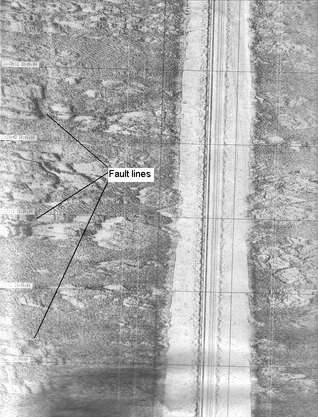
Sample 1 Content: Very fine sediment in a thin oxic layer formed of fine silt/clay, below was a thick dark grey anoxic layer. The pungent odour of oxidized sulphur usually associated within an anoxic sediment, was not very intense and the sediment contained little oil. As expected in this type of sediment there was no life present. A few shell fragments (Mytilus edulis) and leaves were found.

Sample 2 Content:  Very fine clay. There was a higher abundance of life in this grab sample, including a hermit crab, several rocks with calcareous tubes attached to them, nematode worms including polychaetes. A live scallop and a small Crepidula fornicata stack were found. The oxic layer was deeper in this area and able to support more organisms.

GEOLOGY

Sidescan survey 1 was carried out at a start position of 50º20.090N, 004º10.281W.  This transect was started at the edge of Cawsands Bay and continued back and forth from the breakwater, where the average depth of the water is 10-11 metres. The survey speed was 2.5m per second (~ 4 knots). Leading to a survey line time of 10 minutes. Survey 1 continued for an hour, producing 6 lines in total.

Interpretation of Side Scan Sonar Data: It was clear that the southern half of the survey area was mainly made up of constant sediment type, thought to be sand, features in this area were sparse but several strong current ripples were evaluated and found to be around 4cm high. One protruding rock of height 4.3 metres was present, thought to be the consequence to the channel bedrock emerging. Parts of the transect were disturbed by a passing submarine. Further north the data revealed a large dextral fault, amongst the protruding bedrock, several smaller sinistral and dextral faults were also observed (see figure 6). A large sand channel has developed westerly through the northern section interspersed, with ripples and hard substrata. In conclusion it can be seen that a naturally occurring paleo-channel is present due to the flooding of the area at a time in geological history when sea level was lower than it is at present. This deep channel now facilitates the navigation of commercial and navel vessels. The breakwater is also present on the survey, showing an uneven surface, due to an artificial structure interfering with wave processes.

Sidescan survey 2 was carried out at a start position of 50º 21.8580 N, 4º 11.1531W.  Survey lines ran up the estuary covering an area to the east of the first survey line, the end position being 50º 22.1799 N, 4º 11.5711W.  The survey was situated in the estuary channel within the Devonport Naval Base and West Mud, St John’s lake.  The sidescan image shows up two deep channels.  The channel to the north is 264m wide, and extends 39.8m depth at it’s deepest on the south bank.  These channels are divided by a shallow bank which slopes deeply down into the northern channel, with a 20m depth change occurring within a horizontal distance of 5m. The shallow area slopes off more gently into the southern deep channel.  The southern deep channel extends to a depth of 29.7m depth.  The edge of this channel extends over the limit of the survey area. Comparing the side scan image to the Plymouth Harbour and rivers chart, it is clear that survey 2 covers an area crossing the deep shipping channel. A shallower area, called ‘Rubble Bank’ is situated on the inside of the meandering  estuary channel.  The southern deep channel on the survey corresponds to the shipping channel.  This shipping channel then continues to the west.  The second deep channel on the side scan image can be identified as where the shipping channel turns eastwards and crosses the survey area again.  Therefore, in survey 2 we fail to cover the area where the shallow bank slopes into the shipping channel at it’s most westerly extent.  There is no evidence that the ‘Rubble Bank’ area is actually made up of larger clasts than that of the deep channel.  It is possible that the name of this area has historical origins, and that rubble once deposited in this position has now been covered by more fine grained sediment material.

Other features that can be seen, are possible bedforms appearing within an area extending 133.5m from the northern deep channel boundary.  A dredge mark extends to the north from 50º 21.3375 N, 4 º 11.244262 W, for a distance of 230.4m.

3. RIBS (X:\group10\processed data\RIBS)

Date: 02/07/04 Location: Tamar bridge upstream the river Tamar Weather: 7/8ths overcast cloud cover, rain with sunny intervals. Tides: Cotehele Quay (HIGH (4.2m) 05:34GMT - LOW (0.6m) 11:32GMT - HIGH (4.5m) 17:58GMT) Cargreen (HIGH (4.2m) 05:24GMT - LOW (1.0m) 11:52GMT - HIGH (5.4m) 17:48GMT) Research Vessel: COASTAL RESEARCH, OCEAN ADVENTURE

Water samples were collected at 2PSU intervals from the Tamar Bridge upstream. Group 10 was subdivided into two groups. One group used the OCEAN ADVENTURE and the other group used the COASTAL RESEARCH vessel. At a salinity of  3.88PSU the engine of the COASTAL RESEARCH  failed. We almost died in great agony... Subsequently, the COASTAL RESEARCH was towed back by the OCEAN ADVENTURE which was really disappointing. 

3.1 CHEMICAL INTERPRETATION (X:\group10\processed data\RIBS\Chemical and nutrient)

Mixing Profiles

Silicon showed non-conservative behaviour throughout the estuary. Removal is taking place, which is attributed to biological production and degradation processes (Morris, 1981). Non biological reactions may also contribute to control of estuarine silicate. The greatest removal is between 10-25PSU. As noticed by Morris (1980), silicon removal mainly takes place at salinities lower than 15PSU. Therefore we can confirm that silicon removal is more effective at the lower salinity range.  

Nitrate - salinity relationships are predominantly linear, showing conservative mixing behaviour. Nitrate  concentrations follow the theoretical dilution line. 

Phosphate A rather scattered profile of datapoints was obtained. Potentially, removal is taking place at a salinity of 9-12PSU and 25-30PSU. Is has to be noted that unusual distributions of phosphate in the lower Tamar estuary has also been observed by mommaerts (1969,1970) who has attributed this to pollutant sources arising from urbanized and industrialized regions in and around Plymouth. Morris (1980) found that the distribution of phosphate throughout the estuary was influenced by tributary and anthropogenic inputs in the lower 10km of the Tamar. However, this only had minor local effects on Silicon and Nitrate distributions. There are two outlying points of considerably higher concentrations found at salinities 2 and 5.2. These points are possibly due to human error, either during sampling or laboratory analysis.

3.2 PHYSICAL INTERPRETATION (X:\group10\processed data\RIBS)

Using a YSI 650 MDS multiparameter probe, salinity, temperature, pH, time and oxygen saturation (%) measurements were carried out. These measurements were carried out in surface waters at a depth of 10cm. In terms of temperature, a decrease can be recognized towards the mouth of the Tamar estuary. Similarly, a steady decrease in dissolved oxygen saturation can be recognised. The datapoints fluctuate considerably which is probably due to a calibration difference between the two multiparameter probes. The 2 probes were tested on board the RV Bill Conway and a difference in dissolved oxygen of 27.7% was noted. 

From a biological point of view, high chlorophyll concentrations at the riverine end-member produce more dissolved oxygen compared to low chlorophyll concentrations further down the estuary. Therefore, we expect a direct correlation between chlorophyll vs salinity and dissolved oxygen vs salinity. This hypothesis can be confirmed by looking at the chlorophyll vs salinity graph. In terms of the temperature decrease along the upper part of the Tamar estuary, a number of factors must be considered. Firstly, limited depths of 2-3m will increase the stratification of the water column which facilitates heat uptake. Secondly, blocked streams during intertidal periods will cause the temperature to increase more rapidly. Weather conditions preceding the day of data collection were sunny resulting in warm river runoff, a contributing factor to increased temperatures in the upper estuary.  

3.3 BIOLOGICAL INTERPRETATION (X:\group10\processed data\Offshore)

Surface water bottles at a number of locations were collected and filtered. Click here for a Zooplankton and Phytoplankton population changes with salinity graph. 

Phytoplankton Species abundance and distribution: (X:\group10\processed data\RIBS\Phytoplankton)

Surface water bottles at a number of locations were collected and filtered. 

Station	Salinity (PSU)	Total individuals (per ml)	Diatoms (%)	Dinoflagellates (%)	Ciliates (%)
Ribs 13	22.02	79	81	11	8
Ribs 18	28.52	50	77	19	4
BC 15	30.01	47	67	11	22
BC 7	32.3	102.5	74	21	5
BC 17	33.7	135	75	21	4
BC	34.7	136.5	67	11	22

The data presented show that diatoms are the major dominant member of the phytoplankton community in the Tamar Estuary. Over the entire salinity range this overall dominance does not change. This could be due to several possibilities. Diatoms may be the principal primary producer in the estuary, there could possibly be a bloom of diatoms, or possibly their position in the water column is higher than the others as all samples were from the surface. The next most dominant species are the dinoflagellates. In the areas where they are more dominant than ciliates the dominance is very significant, however there are two areas where ciliates dominate over dinoflagellates and surprisingly these are in the same ratio, but at very different salinities.

Zooplankton Species abundance and distribution: (X:\group10\processed data\RIBS\Zooplankton)

Bill Conway Station 1 (salinity 34.65): Found just inside the Breakwater, Plymouth Sound. The Dinoflagellates are dominant within the sample (2460.06 per m-3). Copepods (380.28 per m-3), Siphoniphores and Appendicularians, Decapod larvae are also numerous compared at the Tamar Bridge .

Bill Conway Station 2 (salinity 28.54): At the Tamar Bridge, concentrations of all the species are reduced compared to those in Plymouth Sound and higher up the estuary at Ribs station 2. The Dinoflagellates are again dominant (204.28 per m-3).  The diversity of species in this area is also reduced.  

Ribs Station 1 (Salinity 28.52):  This sample lies a little up stream of the Bill Conway Station at the Tamar Bridge .  The sample at Ribs Station 1, shows more diversity but still reduced total numbers (399.10 per m-3). The number of Dinoflagellates is reduced (16.63 per m-3) and Copepods are now the dominant species (157.98 per m-3). The Polycheates are the second most abundant (119.18 per m-3) and are at their highest numbers out of the four samples.  The number of fish larvae is also relatively important (33.26 per m-3).

Ribs Station 2 (Salinity 18.00): There is a higher abundance of zooplankton (6155.22 per m-3) than at salinities in the region of 28. Decapod larvae are dominant (2854.59 per m-3). Copepods (2497.77 per m-3), Mysids, Cirripede nauplii and Polychaetes are also abundant.  Dinoflagellates are reduced (59.47 per m-3) and show the lowest values for the four stations.  

Interpretation: Dinoflagellates are dominant at the most seaward station and show reduced numbers in lower salinity waters. In the region at salinity 28 we observe a reduction in the diversity and abundance of species within the sample. The graph of salinity against zooplankton and phytoplankton abundance, show this trend. Copepods become more dominant at lower salinities higher up the estuary. As the abundance of Dinoflagellates falls other species becoming more numerous.   

The plots for abundance against salinity for phytoplankton and zooplankton show a positive correlation. Reduced numbers are observed in the region of 28 salinity.  It could be suggested that this distribution occurs due to species adaptation.  Marine adapted species are more dominant lower down the estuary (Dinoflagellates).  Species adapted to lower salinity, freshwater areas are situated higher up the estuary.  Due to the mixing of saline and saltwater within the estuary, it is possible that a reduced number of phytoplankton and zooplankton are adapted to intermediate salinities. This could be what we are observing in our samples, with fewer species able to survive in the transition region between salt and freshwater communites.

4. OFFSHORE BOAT TRIP (X:\group10\processed data\Offshore)

Date 05/07/04. Location: sampling in the area of Eddystone rocks. Weather: sunny, 1/8th overcast. 

Tides: High Tide  07:58GMT (5.2m) Low Tide 14:05GMT (0.8m) Research Vessel: TERSCHELLING.

4.1 CHEMICAL INTERPRETATION (X:\group10\processed data\Offshore\Nutrients)

Silicon (X:\group10\processed data\Offshore\Nutrients\Silicon - 05.07.04 Offshore)

At station 5, in terms of silicon, a significant surface concentration is present. However, it decreases rapidly to a minimum at a depth of 5-7m. After this minimum, silicon concentrations increase again. The minimum silicon concentration at a depth of 5-7m could potentially be linked to diatom blooms which occur at this depth.  

Nitrate 

All three of the Stations show reduced nitrate concentrations at the surface and increasing concentrations with depth. Station 3 and Station 5 show a marked minimum in nitrate concentrations, between 8 and 15m depth.  This depth corresponds to that of the thermocline.  We can hypothesise that these reduced concentrations occur because of nitrate utilisation by phytoplankton, and now by the dinoflagellates which bloom later in the sequence of seasonal species succession.

Station 6, shows relatively constant increases in nitrate concentrations with depth, but we do not see a marked minimum as seen within the other two profiles.

Phosphate

From the 3 sites chosen for analysis, sites 3, 5 and 6 show distinct changes in phosphate concentration with depth. Sites 3 and 5 show a similar pattern of removal in the first 10 metres, with phosphate concentrations in both then increasing rapidly over the next 10 metres. The surface concentrations are more than four times higher at site 3 than site 5. Unusually, there appears to be removal of phosphate taking place again at 25 metres. At site 6 concentrations of phosphate decrease rapidly from 0.2 umol/litre at the surface to 0.0012 umol/litre at seven metres depth, this atypical extent of phosphate removal could be a consequence of the particularly high diatom concentration in the first 10 metres of site 6.

4.2 PHYSICAL INTERPRETATION (X:\group10\processed data\Offshore\CTDdata)

As the ADCP and the minibat were unavailable, our physical interpretation was restricted to the CTD probe. (DT-2000 FSI Falmouth Scientific Inc.) The positions of data collection are shown by clicking on the following  link. Eddystone Rocks are highlighted with a circle. Three stations of interest will be discussed below: stations 6,5 and 3. Please note that fluorescence units are Volts, not millivolts.

STATION 6 (Figure 10)

Salinity (not shown on graph) is mostly uniform throughout the water column at station six. Fluorescence increases rapidly in the surface layer changing from approximately 1.2mV to 3.5Mv and then decreases at the same rate to 20m depth. This is indicative of a phytoplankton bloom and is present just above the thermocline where nutrient levels are at higher than at surface.

STATION 5 (Figure 11)

Salinity (not shown on graph) is mostly uniform throughout the water column at station six.  Fluorescence increases rapidly in the surface layer changing from approximately 1.0mV to 2.0mv and then decreases at the same rate to 20m depth. This is indicative of a phytoplankton bloom and is present just above the thermocline where nutrient levels are at higher than at surface.

The measurements taken in the tidal stream show a smaller fluorescence change than that in the middle of the sampling sites and the breakwater. At sampling site 5, not only are the physical characteristics of the water column affected by the tidal stream, but due to the proximity of the rocks, the water flows around will be affected.  

STATION 3 (Figure 12)

Salinity again is fairly uniform within the water column at this point, it has been left off the depth profile. This point is quite interesting as the thermocline is not so leveled. The thermocline started at 15m, but instead of it being a well defined thermocline, the temperature continues to decrease down to a depth of 30m. The temperature then remains constant down to the seabed. The fluorescence data at this point in the water column only changes over a range of approximately 0.4mV. The presence of chlorophyll in the water column, especially within the thermocline, suggests that zooplankton will also be present. Being in lee of the tide means that only the rocks are directly affecting the physical, chemical and biological characteristics of the water column at this point.

4.3 BIOLOGICAL INTERPRETATION

Phytoplankton Species abundance and distribution. (X:\group10\processed data\Offshore\phytoplankton)

Station 3 - At station 3 phytoplankton levels are relatively low. At a depth of 25m a phytoplankton maximum is present in relation to dinoflagellates. The maximum phytoplankton concentration is limited to 17.5 diatoms per ml at its maximum.

Station 5 - At station 5 higher phytoplankton levels were recorded than at station 3. The highest phytoplankton concentration was present at a depth of 6m with 46 diatom cells being recorded. There is another increase towards the deeper end of the sample, with the number of diatoms reaching approximately 32.

Station 6 - Station 6 is the most productive station in the dataset. Diatom densities up to 65 per ml were obtained in surface waters. Their concentrations decrease rapidly towards a minimum at a depth of 15m below the surface, but again a pronounced increase is seen from 15m to 50m, with diatom levels reaching 60 cells.

Zooplankton Species abundance and distribution: (X:\group10\processed data\Offshore\Zooplankton)

Station 5A:  This sample was taken passing through the thermocline, between 0 and 20 m depth.  The dinoflagellates are dominant and present at a high abundance compared to at the other two stations (35380.91 per m^-3). Sampling evidently took place within a dinoflagellate bloom situated within the thermocline.  The copepods and siphonophores are the next most abundance.

Station 5B: Sampling below the thermocline shows that the abundance of zooplankton at these depths (25-45m) is significantly reduced compared to those within the thermocline.  The dinoflagellates are still dominant (4803.59 per m-3) but not to the same extent as at 5A.  The copepods more are numerous at depth, as are the appendicularians.

Station 6A:   Again sampling within the thermocline, it can be seen that the dinoflagellates are again dominant, but their abundance (15464 per m-3) is less than half of those found at Station 5.  The Appendicularians and Hydrozoans are more important within the zooplankton than the Copepods at this station. 

Station 6B: The partition of the species within the sample between 25 an 45m depth reflects that found at Station 5B.  The total abundance of zooplankton is reduced, and the dominance of the dinoflagellates (4715.8 per m-3) is again less important. The Copepods (2257.8 per m-3) and Appendicularians show increased numbers within the sample.

Dissolved Oxygen (X:\group10\processed data\Offshore\DisOxy)

Station 3: The % saturation remains relatively stable with depth, with a small negative gradient found between 10 and 20 m depth.  % Saturation ranges from 106% at the surface to 94% at 55m depth.  These values are intermediate compared to those of the other two stations.

Station 5:  High % saturation is seen at the surface (177%).  The % Saturation decreases most rapidly from the surface to a depth of 15 m, reaching 93%.  Values are the lowest for all three stations from a depth of 8m down.

Station 6: The highest dissolved oxygen concentrations are observed at this station, throughout the depth profile with concentrations ranging from 144% at the surface, to 102% at 50m depth.

It is interesting that a reduction in dissolved oxygen % Saturation is seen at Station 5, where the highest zooplankton abundances are observed.  The elevated zooplankton concentrations found within the thermocline at station 5 are situated at the same depth as a reduction in dissolved oxygen.  The lowest oxygen concentrations at depth are also found at Station 5.

5. CONCLUSIONS

A general trend is present in the Tamar Estuary. 

From all the above data gathered on the offshore boat trip, we conclude that seasonal summer stratification accommodates the bloom of varying phytoplankton species over a dynamic timescale. The physical parameters enabled, due to the heating of the water column, and the subsequent development of stratification shows a decrease in nutrients but an increase in biological activity in the upper water column. 

6. REFERENCES

Morris, A.W., A.J. Bale and R.J.M. Howland (1981). Nutrient Distributions in an Estuary: Evidence of Chemical Precipitation of Dissolved Silicate and Phosphate. Estuarine, Coastal and Shelf Science 12: pg 205-216. 

Figure 1 - Group 10.

Figure 2 - The Bill Conway.

Figure 3 - Cliff face at Renney Point.

Figure 4 - Fish used for Sidescan sonar survey.

Figure 5 - Grab 2 content.

Figure 6 - Fault lines from Sidescan survey 1.

Figure 7 - The RV. COASTAL RESEARCH

Figure 8 - The RIB OCEAN ADVENTURE

Figure 9 - Rosette Sampling (5 Niskin Bottles as well as a CTD probe)

Figure Figure 10 - Plot showing Temperature and Fluorescence against depth at the above position offshore from the Plymouth Sound (station 6).   

Figure 11 - Plot showing Temperature and Fluorescence against depth at the above position offshore around the Eddystone Rocks (station 6)  

Figure 12 - Plot to show Temperature and Fluorescence against Depth.

Disclaimer

The views and opinions expressed on this webpage are those of group 10 individuals and are not necessarily those of the University.

TOP