Plymouth Field Course 24th June - 8th July 2004

Group 1 Web Report

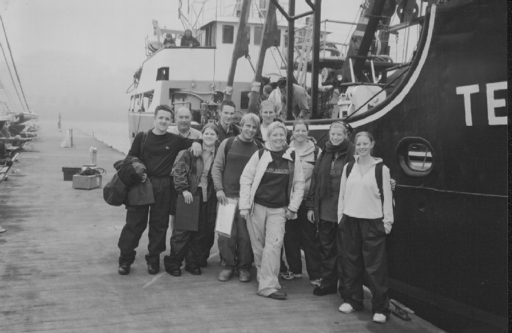
Group 1 beside MV Terschelling at Mayflower Marina, Plymouth. 26th June 2004.

Left to Right: James Bayliss, Simon Boxall (Group Tutor), Jemma Allan, Ed Maxwell, Ben Keen, Paul Stevens, Jenny Jones, Nicke Edge, Kate McNamara, Natalie Crawley

Table of Contents

Introduction

Results and Findings

• Offshore Boatwork

• Estuarine Investigation

• Geophysics Survey

Poem

Click on thumb nailed pictures to view the image full-size

Return to top

INTRODUCTION

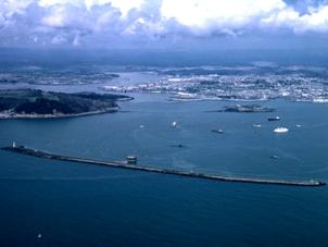
Plymouth Sound including the breakwater, taken from the south-east (www.pml.ac.uk/biomare/sites/plymouth.htm)

The research project was carried out on the south coast in the city of Plymouth. The study region is considered a special area of conservation, where the range in salinity regimes supports a variety of habitats including salt marshes, mud flats and sub-littoral sandbanks. The upper regions of the two main rivers, the Tamar and Lynher, have a well developed salinity system, typical to a partially mixed estuary. The Tamar estuary is 31.7 km long, and is fed by 2 tidal sub-estuaries, the Tavy and the Lynher. The river enters into the Narrows through a 30m deep channel where it then empties into Plymouth Sound (Tattersall, et al., 2003).  There is a 3km long breakwater which protects the harbour from the strong tidal currents of the Atlantic. 

In normal conditions the Sound is well mixed due to its relatively shallow nature, and the Tamar estuary is partially mixed. However, there are areas within the Sound close-by to Drakes Island, which are exceptionally deep (45m) and fill with hyper-saline water from the sea on spring tides.

The research carried out over the two week period investigates stations from the source of the freshwater at the head of the river Tamar, out in the Sound, and past the breakwater extending into coastal seas. Four full marine-based field days and a half-day introduction to the local geology will be used to investigate the holistic interactions of interdisciplinary oceanography and the variations of these over the estuarine and coastal system.    

Return to top | Table of Contents | Next

RESULTS & FINDINGS

Offshore Boatwork

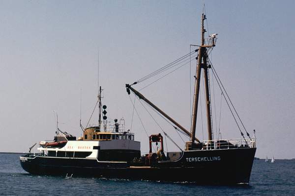
The MV Terschelling in Plymouth Sound (www.shipphotos.co.uk/pages/terschelling.htm)

IN THIS SECTION: Station Details | Aim | Objectives | Station 1 | Station 2 | Station 3 | Station 4 | MiniBAT Tow

* Phytoplankton samples were taken, but subsequently mislaid on the vessel. 

Aim 

To investigate the effects of vertical mixing and stratification on the biological and chemical aspects of offshore coastal waters.

Objectives

Initial Plan

To carry out a shakedown on the east side of the breakwater to ensure the team’s efficiency, equipment is suitably prepared and working correctly to sample further stations. 

Then steam on to Eddystone Rock, to carry out full chemical, biological and physical surveys at four points around the rock, following this, to conduct a continuous survey by circling the rocks towing the MiniBAT.

These surveys are to be carried out with a view to investigate the effect of the physical conditions created by the rocks, focusing particularly on the tidal influence on the biology and chemistry of the water column.

Adaptations

Due to poor weather conditions is was not feasible to sail as far as was initially intended.  As a result four stations, including a shakedown, were sampled allowing a comparison of biological, chemical and physical data of three different environments; offshore, inshore deepwater and water surrounding the breakwater.  Due to the close proximity of the shakedown, Station 1, and Station 3 it is possible to produce a comparison of the breakwater conditions at different tidal states.

Observations and Findings

Station 1 – Shakedown

• Vertical temperature change of 0.5°C.

• Vertical salinity increase is minimal (34.8 – 35.1).

• Although temperature and salinity changes are small, there is evidence from the salinity data that there is significant structure to the water column.  This is seen in Figure 1 where two discrete bodies of water are evident, a warmer, more saline body below with a fresher cooler layer above.

• Chemical data suggests high phytoplankton activity at approximately 3.5 metres where a peak in chlorophyll concentrations and oxygen saturation can be seen.  This corresponds to a decrease in silica concentrations suggesting the presence of diatoms in the water column using the silica to form their skeletal hard parts.

• It should be noted that only three depths were sampled at this station resulting in much of the data being extrapolated, posing questions over the accuracy of these results.

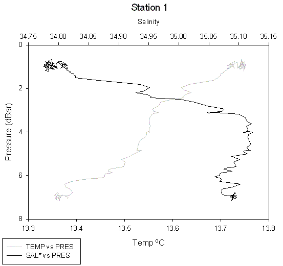
Figure 1: Plot of temperature and salinity against pressure, at Station 1

Station 2 – Offshore

• Figure 2 shows evidence of a seasonal thermocline, with a temperature change from 13.6°C at the surface to 12.4°C at 42 metres.  The presence of high winds and other factors such as headlands, has affected mixing processes creating steps in the temperature, effectively splitting the thermocline in two.

• Heavy rainfall and local run off, causing a significant input of freshwater, has caused a slight dip in surface salinity, resulting in a small halocline being developed.

• Chlorophyll concentrations imply there are more phytoplankton above the thermocline, probably due to stratification.

• For silicon concentrations and Diatom population statistics see Figure 3.  

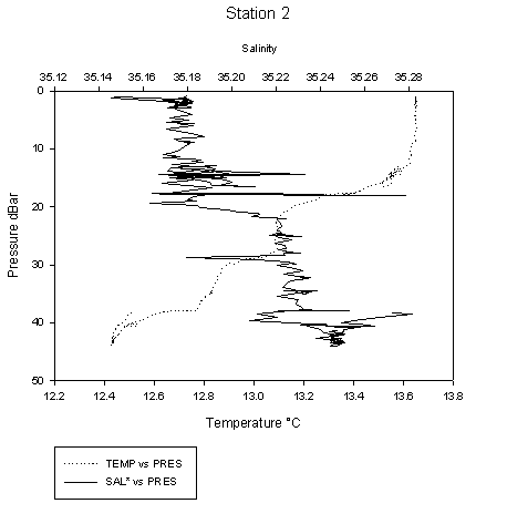
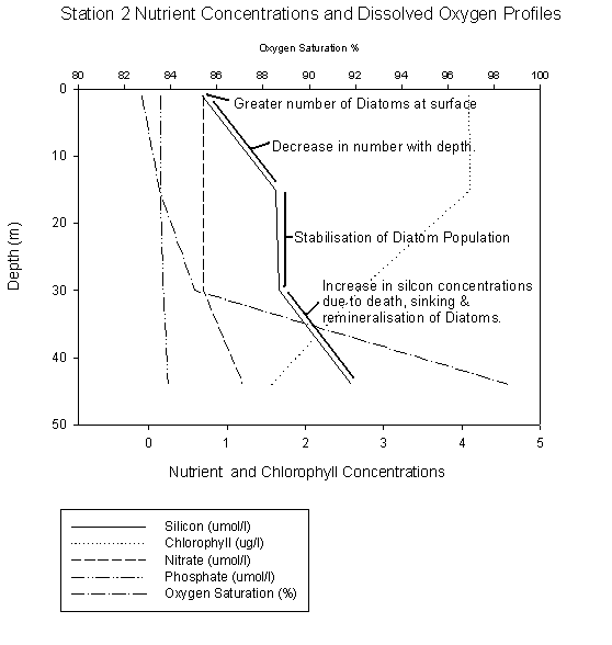
Figure 2: (Left) Plot of temperature and salinity against pressure for Station 2 (click to enlarge)

Figure 3: (Right) Plot of silicon, chlorophyll, nitrate, phosphate and oxygen saturation against depth for Station 2 (click to enlarge)

 Station 3 – Breakwater

• Temperature change 0.1°C suggesting a well mixed water column, also supported by the stability of salinity values.

• Station 3’s temperature is slightly higher than that recorded in the morning at Station 1 due to solar heating during the day.

• When comparing this station with Station 1 it would be expected that when tide is high (morning, Station 1) the salinity would also be highest due the greater tidal influence.  However we found lower salinity in this region due to adverse weather conditions and extremely heavy rain in the morning. 

• The CTD data shows that the chlorophyll concentrations are higher in the surface waters.  However, in the data from the water samples taken, the chlorophyll appears to peak at about 6 metres before the levels begin to drop again.  This indicates that the phytoplankton in the water column have settled around this point.  As expected, these are very similar to the results found at Station 1.

• Silicon levels increase by approximately 1µmol/l through the water column indicating a decrease in the number of diatoms.

Station 4 – Inshore Deepwater

• Temperature decrease from 14.55°C - 14.32°C, salinity increase with depth from 34.1 - 34.37 suggesting a thermodynamically stable water column.  This is reflected in the clear evidence of specific water parcels seen in Figure 4.

• Figure 5 shows more turbidity at the surface due to higher particulate content of the water as a result of run off from rivers and land and higher abundance of plankton and nutrients.

• There is a decrease in chlorophyll at approximately 20 metres, where beyond this depth an increase is apparent.  This is supported by chlorophyll readings from the CTD and is a likely result of turbulence between two bodies of water trapping phytoplankton in the lower layer.

• The zooplankton in this area is dominated by Copepods and Dinoflagellates.

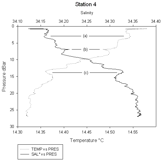
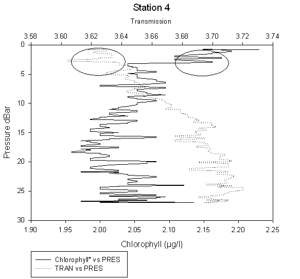
Figure 4: (Left) Plot of temperature and salinity against pressure for Station 4 (click to enlarge)

Figure 5: (Right) Plot of transmission and chlorophyll against pressure for Station 4 (click to enlarge)

Nutrient analysis of Station 4 shows stable nitrate levels, indicating that this is a non-limiting nutrient due to its equal concentrations at the surface and depth.  Similar results can also be seen in the phosphate levels.  Values obtained from oxygen analysis are inaccurate and therefore cannot be used in this discussion.  Stations 1 and 3 have similar results to Station 4.  Station 4 has higher chlorophyll concentrations than at Stations 1 and 3 which would indicate larger populations of phytoplankton and therefore higher numbers of predatory grazing zooplankton.  No comparison of phytoplankton and zooplankton levels can be made for Station 2 due to lack of data collected.

MiniBAT Tow

Position/time of deployment: 50°19.160N, 4°09.110W - 1420GMT

Position/time of recovery: 50°19.820N, 4°08.100'W - 1438GMT

A MiniBAT device was deployed from the vessel south of the breakwater in the Sound and towed for 18minutes to a position adjacent to the eastern end of the breakwater. Since the water was shallow along the length of the transect (from a minimum of 6m to a maximum of 13m, approximately) and high turbulence reduced the efficiency of the flying system, only a limited depth range was sampled. The Surfer software has been used to create shaded plots of temperature, chlorophyll fluorescence and salinity distributions both laterally along the MiniBAT transect and vertically due to the undulating nature of the device.  

For a detailed chart of the MiniBAT tow path, click on the figure 6 thumbnail:

Figure 6: MiniBAT transect path, Plymouth Sound, 26th June 2004

Salinity (Figure 7):

Salinity is seen to decrease along the MiniBAT transect towards the Sound particularly in the surface 4m. This is expected since the estuary is a source of freshwater to the system and is seen as an intrusion in the top right of figure 7 (depicted in yellow). The fresh, warmer water intrusion overlays the saline, colder water due to density variation. As anticipated, the largest salinity values are found further offshore. 

Temperature (Figure 8):

The temperature of surface water decreases as the MiniBAT is towed further into the Sound, from deep water (~13m) to shallow water (~6m) and then back into intermediate water (~11m).  It can be hypothesised that this cooling is as a consequence of wind driven vertical mixing processes occurring in the water column.  These processes create a mixed layer, which is evident to some extent in the temperature depth profiles from Station 2 (offshore), where the seasonal thermocline can be seen to be broken into two main sections separated by a small mixed layer.  As water depth decreases, this layer is forced towards the surface incorporating the warmer surface water and cooler deeper water into it, resulting in a decrease in the surface temperature.  The shallower the water the more pronounced the temperature change is.  Figure 8 strongly supports this theory showing that there is a gradient from the most shallow water (~600secs) where the surface temperature is lowest (13.78°C) to the deepest water sampled(~200secs) where the surface temperature is warmest (13.50°C).  This can also be seen in the representative cross section displayed below.  

Deep water à Shallow water à Intermediate water

Warm surface à Cold surface à Intermediate surface

Chlorophyll fluorescence (Figure 9): 

Fluorescence shows a decrease along the transect with a peak in the deeper, offshore waters (and a slight increase adjacent to the breakwater). The deployment and recovery points (figure 6, points 0 and 8, respectively) were in 10-13m of water whereas the central section was in ~5m of water. In this region, the tidal current creates a layer of turbid water at depth. The peaks in fluorescence correspond to deeper water where the effect of this turbid water is reduced. There is sufficient clear water for high phytoplankton growth and thus chlorophyll-a concentration and fluorescence. This is confirmed by a plot of transmission along the survey. Low transmission corresponds to areas of low fluorescence, particularly at ~600secs. Where fluorescence is highest (at each end of the survey), transmission is high. This also corresponds to the depth profile.

Surfer contour maps of vertical and horizontal distributions of salinity (Figure 7, left), temperature (Figure 8, centre) and chlorophyll fluorescence (Figure 9, right)

Return to top | Table of Contents | Results and Findings | Next | Previous

Estuarine Investigation

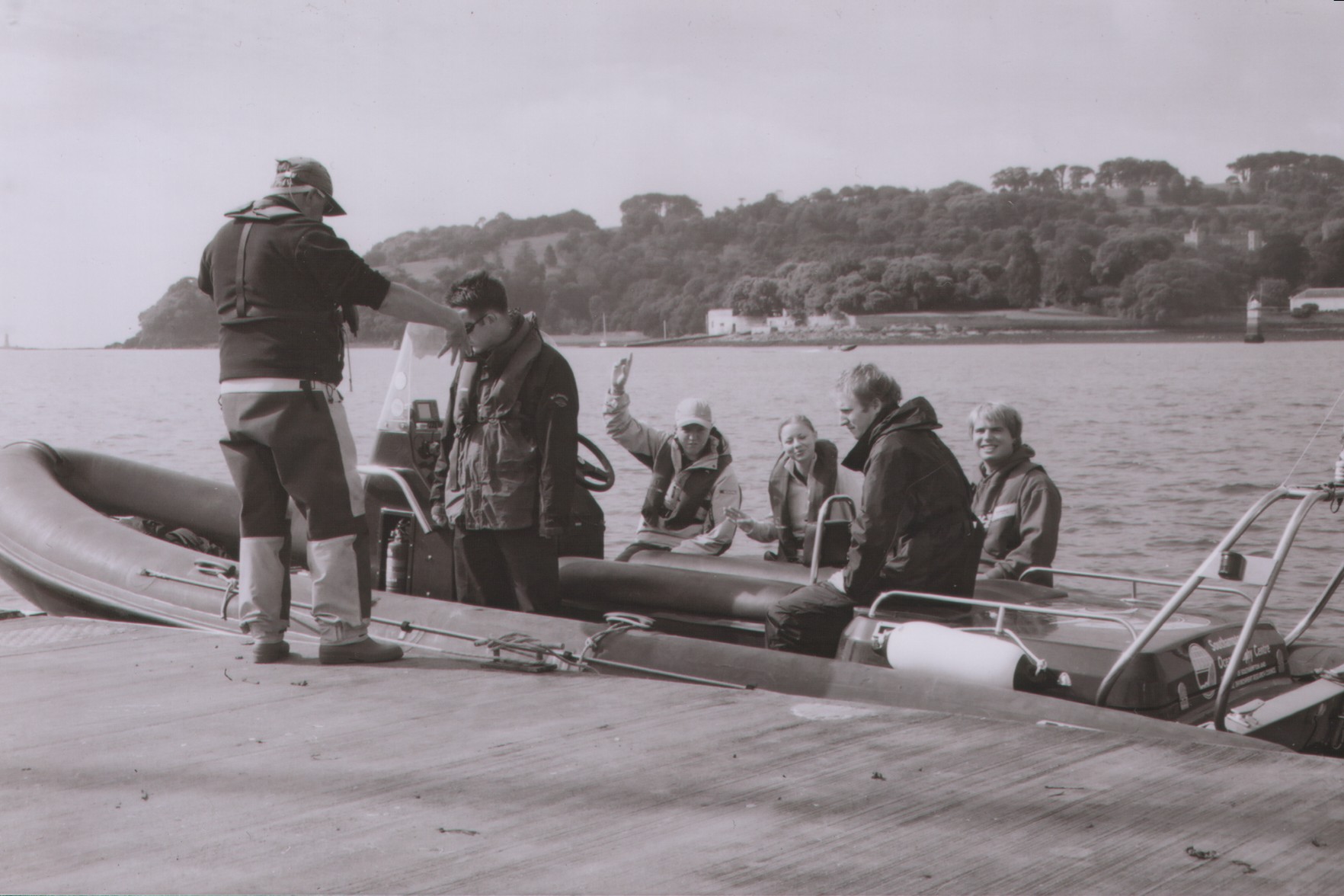
Members of Group 1 on Ocean Adventure: (L-R) James Bayliss, Nicke Edge, Natalie Crawley, Paul Stevens, Ben Keen

IN THIS SECTION: Ribs Station Details | Aim | Method | Physical | Chemical | Biological

Bill Conway Station Details | Aim | Method | Physical | Chemical | Biological | Sound ADCP

Upper Estuary (Ribs)

Details of sampling stations can be found here

Aims

To investigate the physical, chemical and biological processes occurring within the upper Tamar estuary.  Investigation of the mixing behaviour of nutrients and how these are related to the populations of plankton.

Method

A transect study of the Tamar was carried out using 2 small boats.  The first measurements were made at Calstock where the salinity reading was 0.20.  Recordings were then taken at intervals of 2 salinity points so as to gain an accurate representation of the following parameters; surface temperature, salinity, dissolved oxygen, pH and concentrations of the dissolved nutrients nitrate, phosphate and silicate as well as recording the chlorophyll concentration levels.  The vertical profile of temperature and salinity was measured at each station at approximately 1m intervals.  Three zooplankton net trawls were carried out in areas where salinity was 20, 28 and 32.  These samples were processed in the lab to identify the species inhabiting the estuary.  

Observations and Findings

Physical

The depth profiles were analysed using Surfer to produce the transect plots shown below.  The temperature and salinity data were plotted against surface salinity, as opposed to distance along the estuary; this is in order to reduce the effects of sampling different locations, at different tidal states.  

The temperature distribution (Fig.10.) shows a well-mixed upper estuary at salinities <27.  At S>27 there is some  thermo stratification and partial mixing (Fig.10).  Fig.11. also shows a well-mixed upper estuary with: near-vertical salinity contour lines at salinities <27; and stratification at salinities >27.  These data indicate that, at the time of sampling, the Tamar was well-mixed.  However, the Tamar has been described elsewhere as a partially-mixed estuary (Uncles et. al., 1983). 

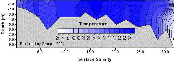
Figure 10: Contour plot of temperature, in relation to surface salinity

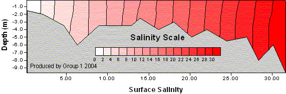
Figure 11: Contour plot of salinity, in relation to surface salinity  

Chemical 

Both phosphate and nitrate are essential nutrients to the growth and reproduction of phytoplankton.  In estuaries, nutrients mix from riverine concentrations to ocean end-member concentrations.  A nutrient that mixes conservatively experiences no net addition or removal during the mixing process.  This causes the nutrient to mix linearly with salinity change, a characteristic that can be represented by the theoretical dilution line (TDL).  Non-conservative behaviour is characterised by non-linear dilution and deviation from the TDL.

Phosphate mixing in the estuary was non-conservative (Figure 12) at salinities between 0 and 10, where data below the TDL indicated net removal from the estuary.  The net removal in the upper estuary correlates to high concentrations of chlorophyll-a at salinities <12.  Data from where salinities >22 indicated net addition of phosphate to the estuary.  This observation could be caused by anthropogenic inputs from built-up areas on the banks and pastoral farms.

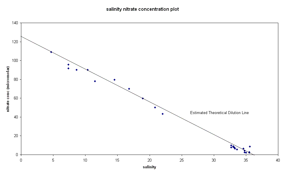
The values for nitrate between riverine and ocean end-members lie below the TDL (Figure 13).  Thus showing that NO₃ is removed from the water, and therefore behaves non-conservatively, due to plant/phytoplankton uptake.

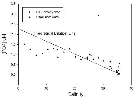
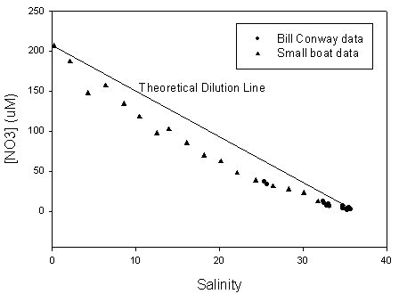
Figure 12 (right): Nitrate in relation to Salinity. Figure 13 (left): Phosphate in relation to Salinity     

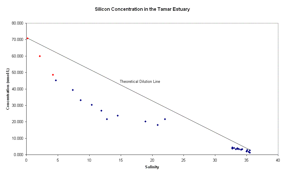
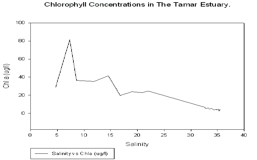
Silicon also behaves non- conservatively within the Tamar estuary (Figure 14).  Silicon is an essential nutrient that is essential for the production of frustules (tests) of diatoms species.  It is probable that Si is removed from the water by these species for growth and this hypothesis is supported by the high diatom numbers at salinities below 12 (Figure 15).  

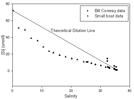
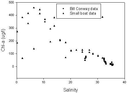
Figure 14 (left): Silicon in relation to salinity. Figure 15 (right): Chlorophyll in relation to salinity

Biological

The phytoplankton community structure shows variability at different salinities, with Diatoms being most common and dominating these samples at low salinities (10 and 12) and high salinities (30 and 35).  At the intermediate salinities (21 and 25), the phytoplankton population is more evenly distributed, with the presence of Dinoflagellates being more common (Figure 16a-g).

The overall numbers of phytoplankton in the intermediate samples are lower (100-150 cells/ml) than at the low or high salinities (200-300 cells/ml).  This is typical mid-estuarine data because intermediate salinities have very stressful environmental conditions caused by fluctuations in pH and salinity.

An abundance scale for the zooplankton was used with the following values:

0-3 per m³ -   normal

3-10 per m³ - common

>10 per m³ -  very common

In the most saline sample (S=32) Cerripede nauplii (dominant), Hydrozoans and Copepods were very common. 

Copepods dominate the least saline sample (S=20).  Dinoflagellates, Cladocerates and Mysidarians are common in the least saline sample. 

The intermediate salinity zooplankton sample shows similar character to the phytoplankton sample, having fewer total animals than the high or low salinity samples and having the highest proportion of dinoflagellates (Figure 18a-c).  Cerripede nauplii are not present in the intermediate or least saline samples, possibly because the Cerripede nauplii are intolerant to water of low salinity.

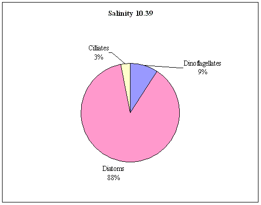
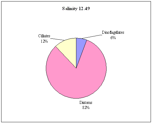
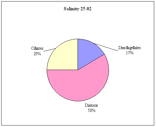
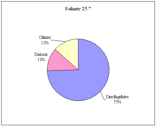
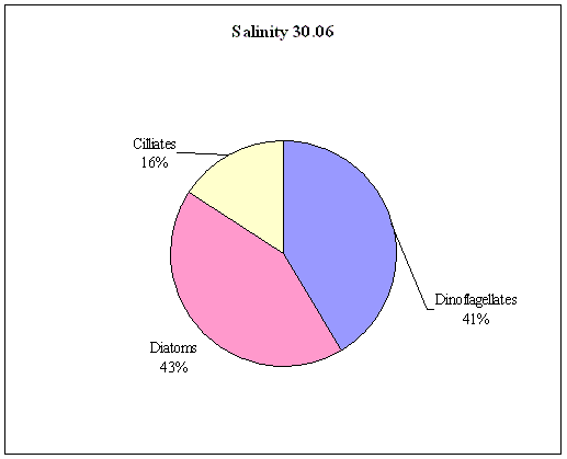
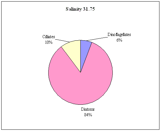
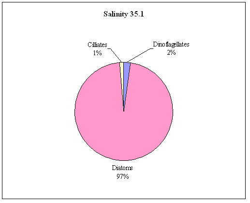
Figure 16a-g: Proportion of different phytoplankton groups in samples over salinity range 10 to 35.1

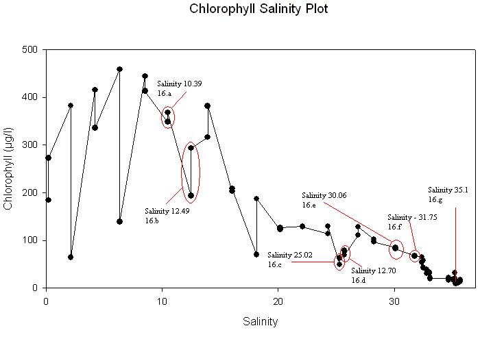
Figure 17: Chlorophyll a salinity plot with phytoplankton and zooplankton sampling sites marked

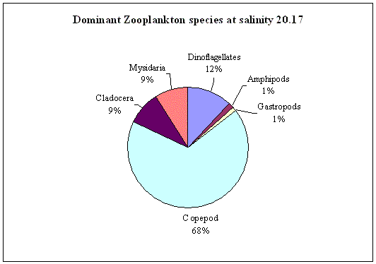
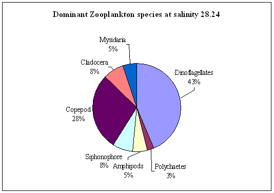
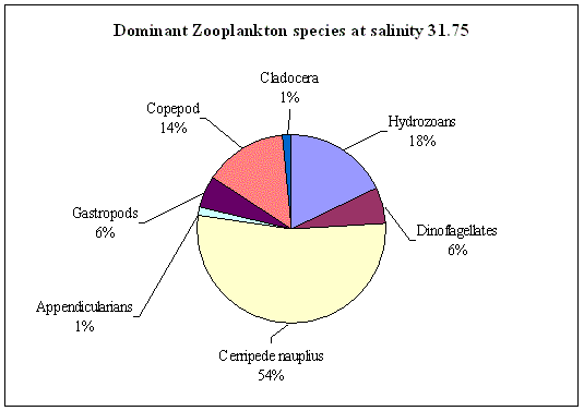
Figure 18a-c: Proportion of different zooplankton groups in samples over salinity range 20.17 to 31.75

Lower Estuary (Bill Conway)

Details for sampling locations can be found here

Aim  

Bill Conway set out to investigate the saline end of the estuary in greater detail than was possible on the small boats. 

Method

A CTD profile was taken at seven positions around the sound and estuary. Water samples were taken from the Niskin bottles for nutrient, oxygen and chlorophyll analysis.  Depths at which samples were taken were decided after consulting the CTD profile to highlight points of interest.  ADCP transects were recorded at the following positions: across the breakwater, to look at its effect upon flow within the sound.  Another was taken from Mount Batten breakwater to the outskirts of Cawsand Bay , looking at the flow from the Cattewater. A third transect was taken across The Narrows. 

Three further transects were taken across the River Tamar, the River Lynher and just below the confluence of the two rivers to investigate the current and flow patterns of the two rivers into the estuary.  A final ADCP transect was taken under the Tamar bridge to look at its effect upon the speed of flow and mixing.

Observations and Findings

Physical - Tamar/Lynher Confluence  

The river Lynher is a tributary of the river Tamar.  The tidal range of the river is approximately 4nm long.  ADCP transects of the Tamar upstream and downstream of the confluence with the Lynher and of the Lynher itself were recorded.  CTD profiles from the approximately the centre of these transects were taken.

Aims

To investigate the impact on nutrients of the river Lynher input into the Tamar. 

To investigate the mixing processes occurring at the confluence of the 2 rivers.

Results and Findings

The general structure of the water was of an ebb tide with warmer, less saline, high- nutrient water overlying cooler, more saline water with lower nutrients. 

The sample data from river Lynher showed higher levels of NO₃ and PO₄ than the River Tamar above the confluence.  The SiO₄ level in the River Lynher is higher than in the River Tamar.  This input of high- SiO₄ water appears to have no effect on the SiO₄ concentration in the River Tamar, as can be seen by the similarity of data from stations 4&6 (Figure 19). 

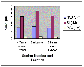
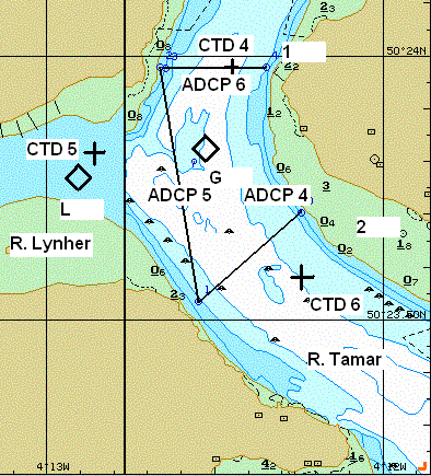
Figure 19 (left): Difference in nutrient concentration at different stations. Figure 20 (right): Chart plot showing ADCP track and CTD location data

This lack of effect is likely however, to be caused by the location of station 6, on the other side of the Tamar to the Lynher.  ADCP data from both of the cross-Tamar transects (ADCP4,6) shows higher flow (0.6ms^-1) on the Eastern side of the Tamar than on the Western side (0.3-0.4ms^-1).  This faster-flowing water may not have mixed with the high- SiO₄ water from the Lynher, therefore giving the appearance of missing SiO₄. 

The ADCP and CTD measurements were made between 0940 and 1040GMT; between 1 and 2 hrs after HW Devonport. 

The tidal stream in the River Tamar was observed by ADCP to be ~0.5ms^-1 (~1kn).  This correlates to tidal stream data from tidal diamond G at 0940 and 1040; 158° at 0.5 and 1.2kn respectively.

The scour effect of the fast tidal and river flow on the outside of the bends (Figure 21 - ADCP6) has the effect of cutting the bank causing a steeply-sloping seabed (shown on Figure 20).  Slower flow on the inside of bends allows deposition causing mudbanks (2). 

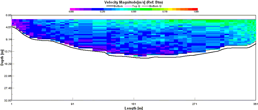
Figure 21: ADCP 6 Magnitude (Tamar above Lynher)

The flow of the River Tamar around the mouth of the River Lynher curved from ~200° to ~130° (Figure 22 - ADCP 5).  The input from the River Lynher entered the Tamar in the Southern half of the confluence.  This can be seen in ADCP 5 from 0-300m where the flow direction shows up blue.  Turbulent mixing of the two water bodies occurs at this point; flow 0.24-0.45 ms^-1 and direction 125°-170°.  This mixing water can also be seen on ADCP4 as a fast, turbulent surface layer.  The Tamar below the confluence appears to be stratified (Figure 23 - ADCP4).  However, the CTD data for below the confluence shows little stratification (CTD6), probably due to the position of the CTD sample, shown approximately on ADCP4 where the water column appears well-mixed.

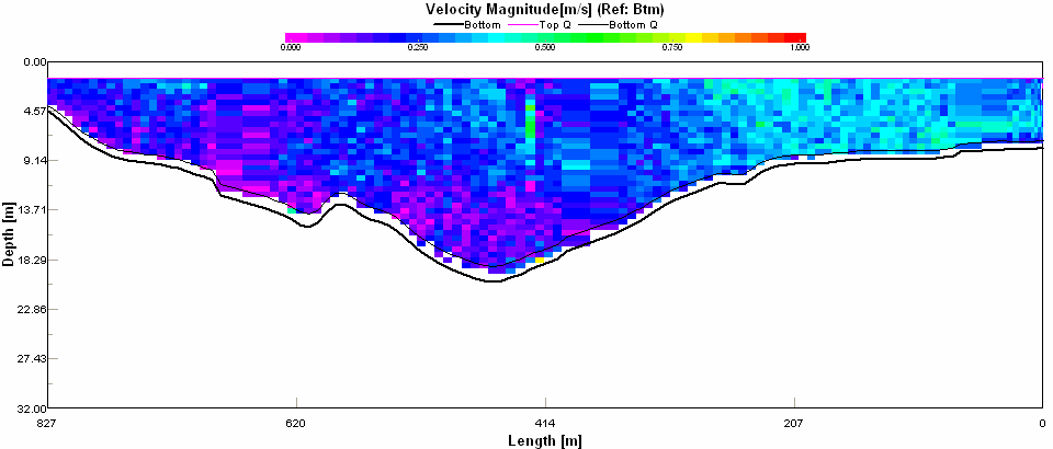
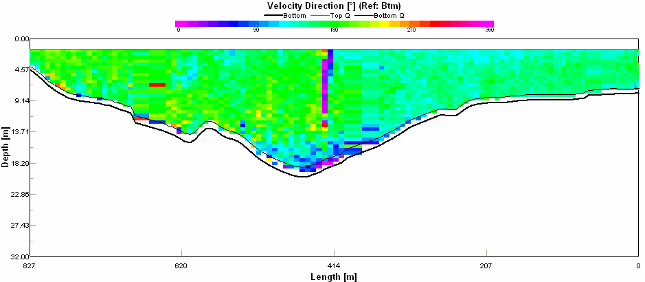
Figure 22: ADCP 5 Flow Magnitude (left) and direction (right)

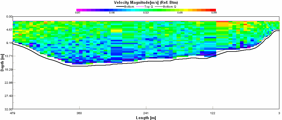
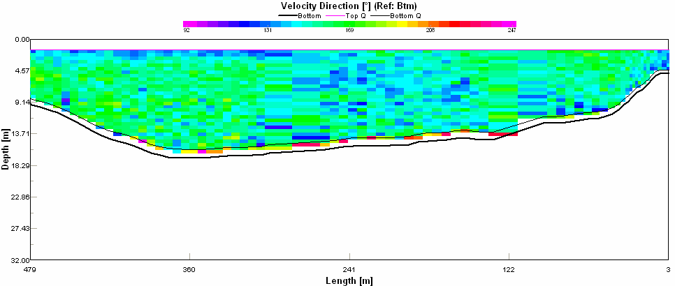
Figure 23: ADCP 4 Flow Magnitude (left) and Direction (right)

The change in direction and magnitude of the inflow (tidal ◊L) at HW+2-5 (~080° at ~1.1kn springs), compared to HW+1 (115° at 0.3kn), may cause an increase in turbulent mixing at the confluence, at other times during the tidal cycle.  The change in direction at HW+2-5 may also cause the turbulent mixing to occur further North in the confluence.

These data are inadequate to draw many firm conclusions from due to the low number of samples, the closeness of the data and the proximity of samples to one another.  For example; the CTD measurement in the River Lynher is too close to the River Tamar to be free of its influence as can be seen in the chart plot.  These data are good enough however, to support the conclusions drawn in this report.

Chemical

The data collected shows the same silicate-salinity relationship as was reported in the small boats analysis.

Figure 24: Silicate-Salinity relationship for the Tamar/Lynher Rivers (red points indicate data taken from Group 1 RIBs 29.06.04)

Figure 24 shows a strong negative correlation between nitrate concentrations and salinity, however, due to data gaps and a high riverine end member salinity value, a TDL could not be drawn.  An estimated TDL was therefore produced, running through an average surface saline end member (35.5) and the sampled riverine end member (4.68).  This line was extrapolated to give an approximation of nitrate concentration of 126 µm at 0 salinity. 

The data obtained suggests conservative behaviour of nitrate, although due to the data gap this cannot be confirmed from these results.  However when compared with data collected by other groups and research conducted by Morris, it would appear that this is a correct assumption. 

Data for salinities that have not been extensively sampled, 0 – 4 and 22 – 32 salinities, have been looked at in more detail using research by Morris.  In the lower salinity range deviation is often observed in the recorded value, however it is short lived and quickly reduced at the higher salinities. Otherwise the plot can be seen to be linear, with short term variability in the composition of freshwater.  It was also noted by Morris that there were “substantial concentration fluctuations were displayed by all three nutrients along the stretch of freshwater immediately above the limit of salt intrusion” and that “Fluctuations produce short term, apparently random, oscillations in nutrient concentrations”. 

Consideration should be taken when using Morris’ data, as it was produced in 1980 and there has been significant changes to an already dynamic environment, for example the removal of a sewage outlet pipe further up the estuary.

Figure 25: Nitrate-Salinity relationship for the Tamar/Lynher Rivers

The data from the small boats practical showed that nitrate was seen to behave non-conservatively (see Figure 4).  This behaviour would be expected more so than conservative, as nitrate should be removed by the high numbers of phytoplankton found in the estuary (Figure 16a-g and Figure 28).  

The oxygen saturation (Figure 25) appears to rise with increasing salinity, this would be expected as there is greater exposure to wind offshore, which will force bubbles formed at the crests of waves down the water column.  The lower oxygen % in regions of lower salinity can be explained by the fact that in riverine areas there is an abundance of detritus causing growth of bacteria, which encourages eutrophication and therefore a decrease in oxygen.

Due to the recent heavy rainfall, it can be suggested that the sudden increase in river volume has caused the detritus to be washed down the river, resulting in evidence of eutrophication at this higher salinity.  It is this that is possibly the cause of there being less oxygen present.

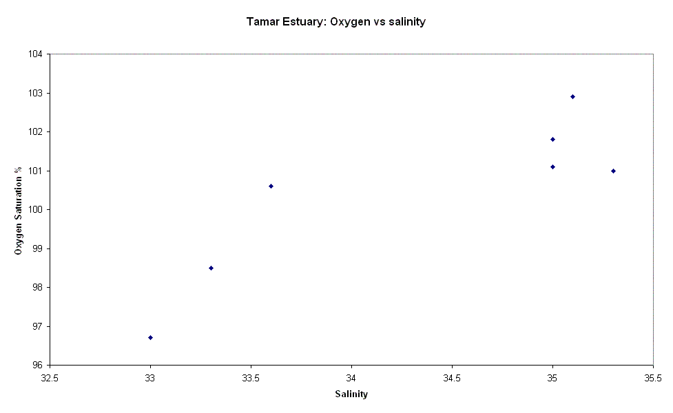
Figure 25: Oxygen-Salinity Relationship for Tamar and Lynher Rivers

Having included values for the lowest salinity points (between 0 and 5) the phosphate-salinity (Figure 26) relationship show that the behaviour of phosphate in the Tamar Estuary can be classified as a non-conservative nutrient.  Phosphate experiences both addition and removal in the estuary, with the removal taking place in the upper estuary, possible due to biological processes by the phytoplankton community.  The addition of phosphate into the estuary occurs in the lower estuary (from salinity 33) before it mixes conservatively out of the estuary.

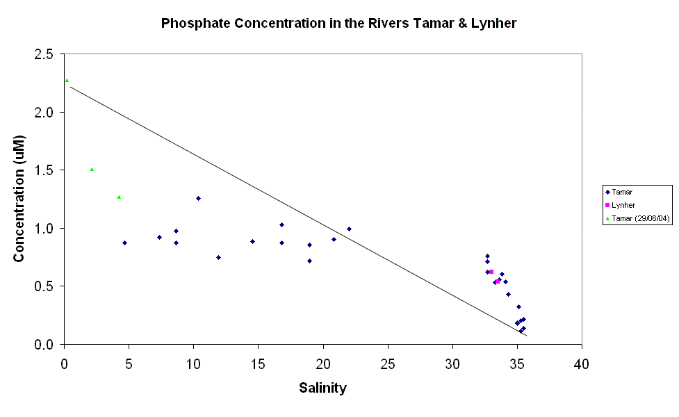
Figure 26: Phosphate-Salinity Relationship for River Tamar and Lynher

Biological

 As suggested by the nutrient data, the most abundant phytoplankton group was the Diatoms, with this group being the most dominant group in all the water samples taken.  Dinoflagellates and Ciliates were present in the samples but not in numbers that would prove to be of any significance to the nutrient data recorded.  From this is possible to suggest that it is the presence of these Diatoms alone that is responsible for the non conservative behaviour of the nutrients in the water column.

The Zooplankton samples an abundance of Cirripede nauplii and Copepods but very small numbers of mature zooplankton organisms indicating that there are unsuitable conditions in this lower salinity region.

 Figure 27: Chlorophyll-Salinity in the Tamar/Lynher Rivers

The data collected on Bill Conway concur with the data collected on the small boats, where chlorophyll concentration (Figure 27) decreases with increasing salinity.  The high chlorophyll concentrations at low salinities correspond with high phytoplankton levels (Figure 28) in more riverine environments.  The highest concentration of phytoplankton was at a salinity of 4, whereas the chlorophyll optimum was at salinity 7.  The fact that the two do not coincide raises doubt into the validity of the chlorophyll.

Figure 28: Phytoplankton populations in the lower Tamar estuary

Reference: Aw Morris, AJ Bale and RJM Howland (1980). Nutrient Distributions in an Estuary: Evidence of Chemical Precipitation of Dissolved Silicate and Phosphate. Estuarine, Coastal and Shelf Science. 12. 205-216.

ADCP Data from Plymouth Sound

ADCP (Acoustic Doppler Current Profiler) transects were made in the Sound at the following locations:  

• West to east across the Sound (north of the breakwater) from 50°20.525N, 004°08.915W to 50º20.578N, 004°07.752W in two sections.

• From Mountbatten Peninsular breakwater (50°21.574N, 004°08.160W) to the Hoe (50°21.752N, 004°08.213W)

• Across The Narrows where the River Tamar flows into the Sound (50°21.596N, 004°10.060W to 50°21.515N, 004°10.253W)

The ADCP transects were carried out at approximately high (slack) water and on the early stages of an ebbing tide. Consequently, flow in the Sound area is low, but is however, still affected by riverine outflows and the complex geometry and bathymetry of the Sound.

The cross-Sound transect shows significant shearing, both between the water column and sea bed and within the water mass as two flows travel in differing directions. A calculation of the Richardson Number in this region (≈0.2) shows turbulence. However, using the simplified calculation for R_i, the result is 1.0. Since this simplified method assumes the greatest shear is with the seabed, the implication is that the shear between water masses is in fact the most significant. We also see the greatest current velocities in the deep water in the centre of the transect (within the dredged channel) and near the far ends of the transect where surface waters flow out of the Sound past the breakwater. Eddying was also noted as the breakwater modifies the main flow of water out of the Sound. This is visible from the stick track for this transect (Figure 29).

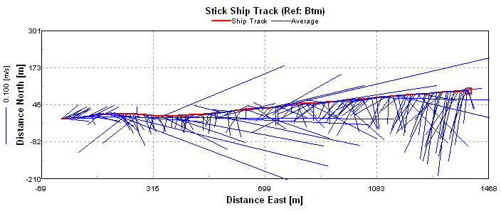
Figure 29: Sitck ship track from WinRiver for the eastern section of the cross-Sound transect, north of the breakwater, showing significant eddying.

The tidal state prevents detailed analysis of the flow regime in the north-eastern section of the Sound (Mountbatten Peninsular to the Hoe – across the Cattewater outflow). The ADCP shows low flow of up to 0.15ms^-1 at all depths and in mostly random orientations (Figure 30). There is some evidence of a westerly flow at the surface and easterly intrusion of seawater at depth.

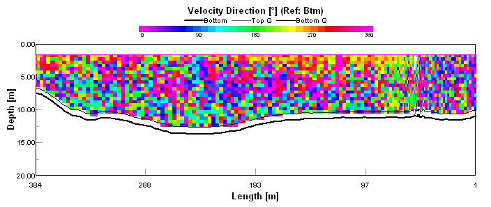
Figure 30: Velocity direction contour from WinRiver showing the random distribution of current flow in the north-eastern Sound

The Narrows ADCP was performed on an ebbing tide, hence the stick plot shows a uniform NW-SE flow (following the direction of the river channel). Current velocities reach a maximum of ~0.5ms^-1 at approx. 5m depth in the middle of the transect since friction is least here. Velocities are ~0.2ms^-1 adjacent to the sea bed.

Return to top | Table of Contents | Results and Findings | Next | Previous

Geophysics Survey

IN THIS SECTION: Aim | Objectives | Results 

Aim

To investigate area of geological interest below the waters of Plymouth Sound, including faulting structures and the distribution of various sediment types.  Also to gain experience using side scan sonar equipment and interpreting data collected.

Objectives

Initial Plan

To run a series of straight transects parallel to the Cawsand coastline, to begin near the breakwater with start and end points of 50°20.170N, 04°11.000W and 50°27.700N, 04°10.800W, respectively. Within this space using a 75m overlap fourteen transects approximately 1 nautical mile in length are possible.  This over lap ensures accurate coverage of the seabed and the length was calculated to incorporate the suspected location of the fault line.  Depending on sea-state three sediment grabs, using a Van Veen Grab, will be taken to confirm the sediment composition at various points within the transects. 

Adaptations

Due to rough weather conditions and sea swell, it was only possible to complete 12 transects in Cawsand Bay. This also prohibited the use of the grab during the transects and as a result the location of the grab survey was executed in a more sheltered area of the bay. A further transect was conducted to incorporate these samples into the acoustic data, running with the coastline. This transect has start and end points of 50°19.980N 04°11.050W and 50°19.990N, 04°11.740W, respectively. The grabs were taken at the following locations:

A transect was conducted through The Bridge (a channel inlet between Drakes Island and the mainland), an area containing very shallow regions, and along side the navel dock walls and an Auxiliary tanker. All of which have been identified on the transect. The acoustic system used has two available frequencies, 100kHz and 500kHz, both of which were used in this transect. The 500kHz frequency gave a more accurate image as it was not affected by the feedback of the Echo Sounder on Nat West II which also uses a frequency of around 100kHz. This course was surveyed as a point of interest and reference rather than for research.

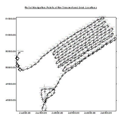
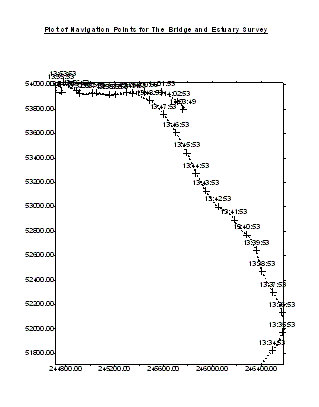
Plots of navigation points for the transects and grab locations (Figure 31, left) and for The Bridge and dockyard survey (Figure 32, right). y-axes and x-axes are GPS-based northings and eastings respectively

Results

The side scan sonar data collected shows lighter and darker patches corresponding to different sediments and surface textures. By placing the transects into a mosaic a distinctive boundary layer runs perpendicular to the direction of the survey track. The dominant sediment type represented by darker shading indicating coarse sediment. The sediment type has been sampled by group 8 and it has been verified to be coarse broken shell. The lighter tone on the transect represents a finer grain material. On a transect closer to the shore, the same feedback was observed, suggesting the same sediment type as seen in the main transects. Three grabs were taken within this track and the sediment collected was a fine sand and mud matrix containing broken shell fragments. Bedrocks formations are present in the north of the surveyed area, closest to the coastline.                                                                                             

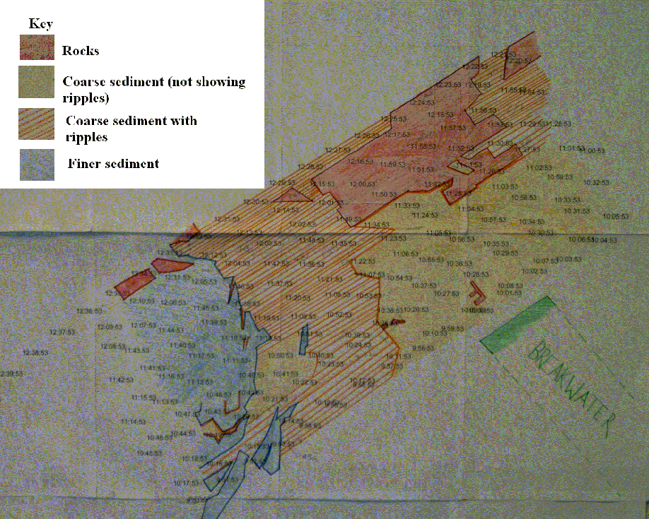
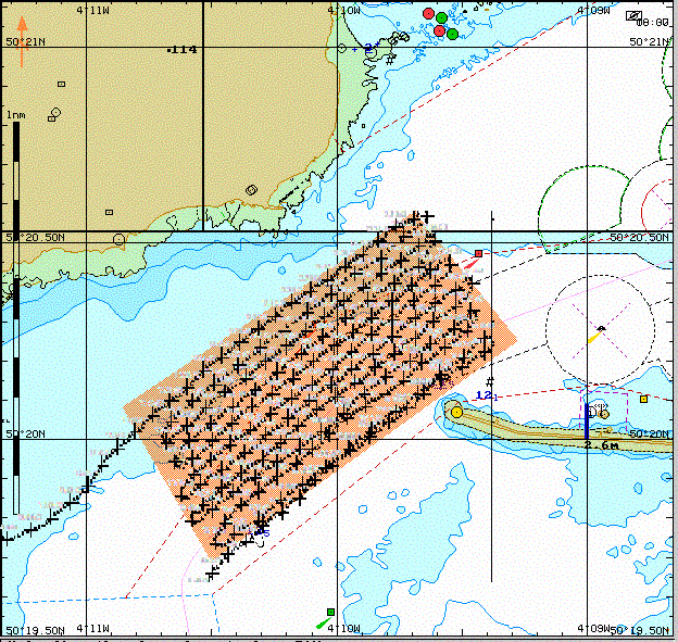
Figure 33 (left): Large-scale plot of Cawsand Bay transect region with sediment types marked as follows: red - bedrock, yellow - coarse sediment, orange striped - coarse sediment with mega-ripples, blue - fine consolidated sediment, green - breakwater (Digital Photo)

Figure 34 (right): Navifisher chart of area surveyed with transects superimposed.

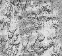
Finer grained sediment 

           Figure 35: Scan of fine sediment from the side scan sonar. 

These sediments comprise of consolidated muds and fine sands with a small amount of broken shells. These do not show any impact from water movement due to strong cohesion of the sediment. This is due to be the compaction of the very smooth, rounded particles that are held in a tight matrix by the pore fluid. This area is larger towards the coast and there is a well defined uneven boundary due to fingers of the coarser grained material. Figure 33 depicts a simplified version of these indents, and there direction indicates flow direction (out of the bay, parallel to the shore). Further out towards the main channel the fine sediment is broken up more by the coarser sediment.

There are no tidal diamonds in the area surveyed; however by using information for the north and south of the bay, it is possible to gain an understanding of the tidal flow in the Cawsand area. The data for these tidal diamonds show the ebb tide flows over a greater period of time, towards the headland. As a result it is then deflected round to produce an eddy, which is also contributed to by the strong tidal flow across the mouth of the sound (Figure 34). The strong ebb causes a faster flow in the south west area of Cawsand Bay, this correlates with the area of finer sediment on the side scan sonar data. Deposition of the coarser grain material occurs in the slower flowing regions. The presence of this eddy could explain the pattern of fine and coarse sediment, and the direction of the finger indicates the south easterly tidal flow in that area, as it is deflected by the ebb tide flowing from north of the breakwater.

Coarse grained sediment 

             Figure 36: Coarse grained sediment showing ripples from the side scan sonar

This area is composed of broken shell, and is split into two sections. One section contains ripples and the other section showed a flat bed with no obvious structure. The average wavelength of the ripples is 1.3m and can therefore these ripples can be classified as megaripples. This classification is based on the characteristic wavelength of megaripples which, 0.6m – 20m (Amos 2003).  The rippled areas are represented on the plot (Figure 33.) by orange lines, which indicate the orientation of the ripple crests. These ripples run parallel to the shore which suggests the tidal currents are perpendicular to the coastline.

The boundary between the rippled and non rippled area may be influenced by the position of the Breakwater and the presence of bedrock. Also having viewed a bathymetric plot of the area surveyed, produced by students from the University of Plymouth, a correlation between water depth contours and the boundary could be seen. The boundary coincides with a deeper section of water, not shown on the hydrographic chart. The increased depth causes the surface waves to have a lessened impact on the sea bed so therefore no ripples are produced. Also the position of the bedrocks will lift flow produced by the eddy, reducing the impact it has on the sediment, and the ebb flow out of the bay will deflect the flow out of this area. The ripple crests have formed parallel to the shore due to the eddy formation in the bay mentioned above.

Bedrock

                Figure 37: Bedrock formation from the side scan sonar

The bedrocks are a submarine extension of the headland Picklecombe Point, these have not been analysed in depth, a simplified version has been plotted (Figure 33) to shows the perimeter. This bedrock is also interlaced by deposits of coarser sediment. The presence of these rocks disturbs current flows causing increased turbulence and therefore re-suspension of the sediment into the water column.

References: Amos, C. L. 2003. SOES2009 Lecture Notes (Lecture 9 Estuarine bedforms) 

Return to top | Table of Contents | Results and Findings | Next | Previous

And to close... the Group 1 poem by Ken Been

Hard at work but having fun

We're the guys of AWESOME Group 1

Two weeks of working, we're going mad

Out on the boats, weather's always bad

In the labs with white coats on

Getting all the plankton wrong

Simon standing on the stern

Ken and Kate catching carp

Paul perusing the port

And Ed examining Eddystone

Nicke and Natalie naughtily nattering

Jemma and James juggling jellyfish

With Jenny jabbering gibberish

The site wouldn't be complete without a few of the best Group 1 quotes: 

"Four thingy grams per wotsit" (Kate)

"My foot doesn't feel like my foot, it feels like my other foot" (Jemma)

"Stop it! You're getting the equipment wet" (Ed)

"I feel stoned" (Ben)

"I used to live in Cypriot Cyprus" (Kate)

"You ought to listen to 'Big Love' by Lindsey Davenport" (Ben)

"FRO" (Nicke)

"I like your hat" (Kate)

"I be a mushroom. I be left in the dark and fed on shit" (Graham)

"Poo on a stick" (Nicke)

Group 1 - Plymouth Field Course 2004